Qualcomm Interview Prep — 05. Camera, ISP, Imaging & Multimedia¶
Scope. Everything from photons to pixels to encoded video: the image sensor and MIPI link, the ISP pipeline end-to-end (black-level → lens-shading → demosaic → white-balance → denoise → color-correction → gamma/tone-map → sharpen → color-space), 3A (AE/AF/AWB), multi-frame HDR & night mode, noise reduction, classic image-processing ops (interpolation, masking, edge detection, segmentation, face detection), color spaces (RGB/YUV, 4:2:0), the Android camera stack (Camera2/HAL3/CamX), video codecs (H.264/HEVC, I/P/B frames, rate control), and Qualcomm Spectra ISP context. Pure C/pointer mechanics live in
01_c_programming.md; C++/OOP (vtables, RAII) in02_cpp_oop.md; algorithm/complexity theory (KMP, BFS/DFS, sorting) in03_dsa.md; OS sync primitives (mutex/semaphore/reader-writer, scheduling) and virtual memory in04_os.md; CNN/ResNet/object-detection ML in06_ml_deeplearning.md; kernel drivers/V4L2/ioctl/DMA in07_embedded_linux_kernel.md; aptitude/puzzles in08_logical_puzzles_aptitude.md; number representation/digital-design/pipeline-hardware in09_computer_arch_digital_design.md; the screen-tearing / frame-buffer LLD in10_lld_system_design.md; project/behavioral framing in11_behavioral_hr_projects.md. Overlaps are cross-linked, not duplicated.How to read each entry. Every question is answered in layers so you can stop at the depth you need: - Q — the question, phrased as interviewers actually ask it. - Frequency — how often it showed up in the 75 collected reports (tier + approximate count). - Concept — the basis — book-style fundamentals with worked examples and, where it helps, an SVG diagram. - The "wh"s — Why it exists (what problem it solves), Where you see it (real Qualcomm camera/ISP/multimedia situations), and any important caveat. - Answer — a tight, say-it-out-loud interview answer. - Solution / good example — for "how do you implement/design/debug X" questions, a complete, copy-pasteable code or design. - Follow-ups / gotchas — the traps interviewers spring next. - Seen in — the source reports.
Terms in bold-italics like demosaic, Bayer CFA, 3A, chroma subsampling, rolling shutter are defined in the § Encyclopedia at the bottom — search there for any keyword.
Frequency legend (sample = 75 collected interview reports; counts are approximate and partly from aggregator pages, so treat them as directional): 🔥🔥🔥 Very common (~8+ reports) · 🔥🔥 Common (~4–7) · 🔥 Occasional (~2–3) · ◽ Foundational (rarely asked verbatim, but assumed and underpinning everything else).
Why camera/ISP dominates the imaging loop. Qualcomm's camera/ISP/multimedia loop runs five-plus rounds spanning image-processing + ISP architecture, C/C++ embedded, camera driver + Android HAL, and a cross-functional round with the sensor/apps team. The CleverPrep aggregated guide and the JoinTaro/GeeksforGeeks reports show the domain questions are remarkably stable: explain the ISP pipeline, implement AE, design noise reduction, explain HDR, debug a green tint, design a multi-sensor driver, explain 3A, explain night mode, design a low-latency preview, and discuss the IQ-vs-speed trade-off. This file covers each of those plus the image-processing fundamentals (interpolation, masking, edge/face detection, segmentation), color spaces, and the video-codec questions. Evidence base: qualcomm_camera_interview_experiences.md.
Table of contents¶
- A. Image sensor & the link — A1 sensor basics & Bayer CFA · A2 rolling vs global shutter · A3 MIPI CSI-2
- B. The ISP pipeline — B1 pipeline end-to-end · B2 black-level & lens-shading · B3 demosaic/debayer · B4 color-correction matrix · B5 gamma & tone mapping · B6 color-space conversion
- C. 3A — the control loops — C1 what is 3A · C2 auto-exposure (implement it) · C3 auto-focus (contrast/PDAF) · C4 auto-white-balance (gray world) · C5 debugging a green tint
- D. Computational photography — D1 multi-frame HDR · D2 noise reduction (spatial/temporal) · D3 night mode · D4 interpolated frame between two images · D5 IQ vs speed trade-offs
- E. Classic image processing — E1 interpolation (bilinear/bicubic) · E2 edge detection (Sobel/Canny) · E3 masking & convolution · E4 face detection · E5 image segmentation · E6 multidimensional images · E7 the image-processing workflow
- F. Color spaces & data — F1 RGB vs YUV & 4:2:0
- G. The Android camera stack & drivers — G1 sensor→ISP→driver→HAL→framework→app · G2 Camera2 / HAL3 / camera3 ops · G3 multi-sensor driver architecture · G4 low-latency preview pipeline
- H. Display & video — H1 screen tearing & frame buffers · H2 video bit-rate / rate control · H3 codecs (H.264/HEVC, I/P/B, motion estimation)
- I. Qualcomm Spectra context — I1 what is the Spectra ISP
- § Encyclopedia — searchable glossary
- § Last-5-minutes cheat sheet
A. Image sensor & the link¶
A1 · Q: How does an image sensor work, and what is the Bayer pattern?¶
Frequency: 🔥🔥 Common — assumed in every camera/ISP round; the Bayer CFA underpins demosaic, AWB, and the whole RAW pipeline.
Concept — the basis. A digital image sensor (CMOS today, historically CCD) is a 2-D array of photodiodes. Each photodiode is a "photon bucket": incoming light frees electrons (the photoelectric effect), accumulating charge proportional to the light that hit that pixel during the exposure. After exposure, that charge is read out, amplified (analog gain = ISO), and digitized by a per-column ADC into a number. A bare photodiode is colorblind — it measures intensity, not color. To get color, a color filter array (CFA) is bonded over the pixels so each pixel sees only red, green, or blue light. The dominant CFA is the Bayer pattern: a repeating 2×2 tile of R G / G B, i.e. 50% green, 25% red, 25% blue.

Example — why twice as many green:
Bayer 2x2 tile          Sampling rates
  R  G                  Green: 50%   (luminance carrier)
  G  B                  Red:   25%
                        Blue:  25%
Why it exists. A sensor pixel can only measure how much light, not what color. You could use three sensors + a prism (3-CCD, used in some pro video) but that's bulky and expensive. The Bayer CFA is the cheap, compact answer: one sensor, a mosaic of color filters, and software (demosaicing, B3) to reconstruct the two missing colors at each pixel. The output of the sensor is therefore a single-channel RAW mosaic, not a full RGB image.
Where you see it (Qualcomm). Every phone main/ultrawide/tele sensor is a Bayer (or Bayer-derivative: Quad Bayer / Tetracell, where 2×2 same-color pixels bin together in low light). The ISP's first job is to consume this RAW Bayer stream. PDAF pixels (C3) are embedded in the Bayer grid. Understanding "RAW is one color per pixel" is the prerequisite for every later question.
Answer. "An image sensor is a grid of photodiodes; each converts light to charge that's amplified and digitized. Photodiodes are colorblind, so a Bayer color filter array — a 2×2 RGGB tile, 50% green, 25% red, 25% blue — sits over them, with extra green because green carries luminance and the eye is most sensitive to it. The sensor outputs a single-channel RAW Bayer mosaic; the ISP then demosaics it into full RGB. Modern sensors add Quad-Bayer binning for low light and embedded PDAF pixels for focus."
Follow-ups / gotchas. RAW is linear in light (before gamma) — that's why black-level/lens-shading/white-balance happen in RAW. Bit depth matters: 10/12/14-bit RAW vs 8-bit display (Qualcomm's Spectra is 18-bit internally). Other CFAs exist (X-Trans, RGBW, RYYB) but Bayer dominates. Dynamic range is limited by full-well capacity (saturation) and read noise (floor). Cross-link: bit depth / ADC → 09_computer_arch_digital_design.md.
Seen in: CleverPrep camera guide (ISP pipeline "from raw sensor data"); GfG Graphics SWE ("general image processing workflow", "multidimensional images"); standard image-sensor expectation.
A2 · Q: What is the difference between rolling shutter and global shutter?¶
Frequency: 🔥 Occasional — a sensor-fundamentals probe; explains motion/HDR artifacts.
Concept — the basis. The shutter decides when each pixel integrates light. - Global shutter: all pixels start and stop exposure at the same instant, then the whole frame is read out. No motion skew — a spinning propeller looks straight. Costs more transistors/pixel (a per-pixel storage node), so it's larger/pricier and historically noisier. - Rolling shutter: pixels are exposed and read out row by row, top to bottom, each row slightly later than the one above. Cheap and standard in CMOS phone sensors — but because the bottom of the frame is captured milliseconds after the top, fast motion produces skew/jello (a vertical pole leans), and a flash or flicker can band the image.
Example — the rolling-shutter artifact:
Fast-moving vertical pole, rolling shutter (top read first):
  row 0   |          ← pole was here
  row 1    |
  row 2     |         ← pole moved right by the time this row was read
  row 3      |
            → result: a straight pole appears slanted ("skew")
Why it exists. Rolling shutter is a consequence of cheap CMOS readout: you can't afford per-pixel sample-and-hold for billions of pixels, so you read sequentially. Global shutter solves motion fidelity at hardware cost; it matters for machine vision, fast action, and synchronizing with strobes.
Where you see it (Qualcomm). Rolling-shutter skew is a real problem for multi-frame HDR and video stabilization — the ISP/algorithm must model the per-row time offset to align frames. Flicker from 50/60 Hz lighting causes banding that AE/flicker-detection must cancel. Some Snapdragon camera features assume staggered/rolling readout; XR/AR and high-speed capture push toward global shutter.
Answer. "Global shutter exposes every pixel simultaneously, so there's no motion distortion, but it needs per-pixel storage and is costlier. Rolling shutter exposes row by row, which is cheap and standard in CMOS phone sensors but causes skew on fast motion, wobble during panning, and banding under flickering light. The ISP and HDR/stabilization algorithms have to compensate for the per-row time offset of a rolling shutter."
Follow-ups / gotchas. Rolling shutter also complicates flash/LED sync and HDR (rows captured at different times → ghosting). "Staggered HDR" / DCG sensors mitigate by interleaving exposures. Global shutter ≠ mechanical shutter. Cross-link: timing/pipeline hardware → 09_computer_arch_digital_design.md.
Seen in: Standard sensor expectation (camera/ISP architecture round); relevant to HDR challenges (CleverPrep) and stabilization.
A3 · Q: How does the sensor get its data to the SoC — what is MIPI CSI-2?¶
Frequency: 🔥 Occasional — driver/HAL and ISP-architecture rounds assume it.
Concept — the basis. MIPI CSI-2 (Camera Serial Interface 2) is the industry-standard, high-speed serial link that carries pixel data from the image sensor to the SoC's ISP. It runs over a physical layer — usually D-PHY (clock + data lanes, differential) or C-PHY (3-phase encoding, more bits/symbol) — using several lanes in parallel for bandwidth. Pixel data is packetized (with line/frame start/end markers and a virtual channel so one link can carry multiple streams). A separate low-speed control bus — I2C / CCI — configures the sensor's registers (resolution, exposure, gain, frame rate).
Example — the two buses:
            ┌─────────── MIPI CSI-2 (D-PHY/C-PHY) high-speed data ──────────┐
  SENSOR ───┤  packetized RAW Bayer, N lanes, 100s of Mbps–Gbps per lane    ├──► ISP
            └──────────────────────────────────────────────────────────────┘
            ┌─────────── I2C / CCI low-speed control ───────────────────────┐
  SENSOR ◄──┤  set exposure time, analog gain, ROI, frame rate, start/stop  ├──  AP
            └──────────────────────────────────────────────────────────────┘
Why it exists. A 108 MP sensor at 30 fps generates billions of bytes/second — far too much for a slow parallel bus, and parallel buses don't scale (skew, pin count, EMI). A few differential serial lanes carry that bandwidth with few pins and good signal integrity. Splitting control (slow I2C) from data (fast CSI-2) keeps the design clean: you tweak exposure over I2C while frames stream over CSI-2.
Where you see it (Qualcomm). The camera driver brings up the CSI-2 receiver (CSID/CSIPHY blocks), configures lanes/data-types, and routes the stream into the ISP; the sensor sub-driver pokes the sensor over CCI/I2C. Lane count, data type (RAW10/RAW12), and virtual channels are exactly the knobs a multi-sensor driver (G3) juggles.
Answer. "MIPI CSI-2 is the standard high-speed serial interface that streams pixel data from the sensor to the SoC's ISP, typically over a D-PHY or C-PHY physical layer with several lanes for bandwidth and virtual channels to multiplex streams. Sensor configuration — exposure, gain, resolution — goes over a separate slow I2C/CCI control bus. It exists because modern sensors produce gigabytes per second that a parallel bus can't carry cleanly; serial differential lanes scale better."
Follow-ups / gotchas. Virtual channels let one CSI-2 link carry several logical streams (e.g. image + embedded metadata + PDAF). Data types encode the bit depth/format (RAW10, RAW12, YUV422). The ISP sits right after the CSI-2 receiver. Cross-link: kernel V4L2 sub-devices, ioctl, DMA buffers → 07_embedded_linux_kernel.md.
Seen in: Camera ISP Architecture loop (Part B: "pipeline architectures, timing constraints"); driver-architecture question (CleverPrep, Report 15 kernel↔HAL); standard MIPI expectation.
B. The ISP pipeline¶
B1 · Q: Explain the ISP pipeline from raw sensor data to final image output.¶
Frequency: 🔥🔥🔥 Very common (the single most-asked camera-domain question; the CleverPrep camera guide lists it first and the "review ISP pipeline stages" tip repeats it).
Concept — the basis. The ISP (Image Signal Processor) is the fixed-function hardware block that turns the sensor's noisy, single-channel RAW Bayer mosaic into a clean, viewable RGB/YUV image. It's a streaming pipeline: pixels flow through a chain of stages, mostly line-by-line, with a parallel 3A statistics engine feeding a control loop. The canonical order (verified against vendor/patent pipeline descriptions) is:

- Black-level correction (BLC) — subtract the sensor's "dark" pedestal so true black reads as 0. (B2)
- Lens-shading correction (LSC) — multiply a per-pixel gain to fix vignetting (corners darker than center) and color shading. (B2)
- Defective-pixel correction + RAW denoise — replace stuck/hot pixels; pre-clean RAW noise.
- White balance (AWB gains) — scale R and B (relative to G) so neutrals look neutral under the scene's illuminant. (C4)
- Demosaic / debayer — interpolate the two missing colors at every pixel → full RGB. (B3) This is the RAW→RGB boundary.
- Noise reduction — spatial/temporal denoise on the full-color image. (D2)
- Color-correction matrix (CCM) — a 3×3 matrix mapping sensor RGB to a standard color space (sRGB). (B4)
- Gamma / tone mapping — compress the linear high-dynamic-range data into a perceptual/display curve. (B5)
- Sharpening / edge enhancement — boost local contrast at edges.
- Color-space conversion — RGB → YUV 4:2:0 for encoding/preview. (B6, F1)
The key principle: corrections that depend on linear light and on the Bayer layout happen in the RAW domain (before demosaic); color/tone/perceptual operations happen after you have full RGB.
Why it exists. RAW sensor output is unusable directly: it has a black pedestal, lens vignetting, dead pixels, a strong color cast (sensor spectral response ≠ sRGB), heavy noise, and only one color per pixel. Each ISP stage removes one defect. Doing it in dedicated hardware (not the CPU/GPU) is essential because you must process, say, 3.2 gigapixels/second within a tight power and latency budget — a general CPU couldn't keep up at phone power levels.
Where you see it (Qualcomm). This is the Spectra ISP (I1). Camera-tuning teams spend their lives setting the parameters of each stage per sensor per lighting condition ("IQ tuning"). The cross-functional and ISP-architecture rounds probe whether you understand the order and why — e.g. "why is white balance before demosaic?" or "why is gamma near the end?"
Answer. "The ISP turns the sensor's single-channel RAW Bayer data into a viewable image through a streaming pipeline. In the RAW domain — where data is linear and per-Bayer-channel — it does black-level correction, lens-shading correction, defective-pixel correction and RAW denoise, and applies white-balance gains. Then demosaic reconstructs full RGB. In the RGB/YUV domain it does noise reduction, the color-correction matrix to map sensor color to sRGB, gamma/tone mapping to fit dynamic range to the display, sharpening, and finally color-space conversion to YUV 4:2:0. A parallel 3A statistics engine gathers histograms and focus metrics to drive auto-exposure, auto-focus, and auto-white-balance across frames. The ordering matters: linear-light, Bayer-domain fixes come before demosaic; perceptual color/tone fixes come after."
Follow-ups / gotchas. Exact stage order varies by vendor (BLC and LSC are sometimes swapped; some apply white-balance gains after demosaic; some do a de-gamma/linearization first), so state the principle (RAW-domain vs RGB-domain) rather than memorizing one fixed list. "Why WB before demosaic?" — because demosaic interpolation works better when channels are balanced; also it's cheap per-channel in RAW. "Why gamma late?" — it's a non-linear perceptual mapping; you want to do math (CCM, denoise) in linear light first. Cross-link: fixed-function hardware pipelining → 09_computer_arch_digital_design.md.
Seen in: CleverPrep camera guide ("Explain the ISP pipeline from raw sensor data to final image output", tip "Review ISP pipeline stages (demosaic, denoise, color correction, tone mapping)"); GfG Graphics SWE ("general image processing workflow").
B2 · Q: What do black-level correction and lens-shading correction do?¶
Frequency: 🔥 Occasional — a "do you really know the early stages?" probe within the pipeline question.
Concept — the basis. - Black-level correction (BLC): even with zero light, a sensor pixel reads a small non-zero value — a deliberate pedestal/offset plus dark current. BLC subtracts this per-channel offset so that true black maps to digital 0. If you skip it, blacks look milky/grey and the color-correction math is biased. - Lens-shading correction (LSC): a lens passes more light through the center than the edges, so an evenly-lit white wall comes out darker and color-shifted at the corners (vignetting + color shading, because the falloff differs per channel). LSC applies a per-pixel gain map (low gain at center, rising toward corners) to flatten the field. The gain roughly grows with distance from the lens optical center.
Example — conceptually:
// Black-level correction: subtract pedestal (per Bayer channel Gr,R,B,Gb)
out = clamp(in - black_level[channel], 0, max);

// Lens-shading correction: multiply by a smooth gain map (brightens corners)
out = clamp(in * lsc_gain[x][y], 0, max);   // lsc_gain≈1.0 center, >1.0 corners
Why it exists. These are sensor/lens physics corrections that must happen in linear RAW before any color math. BLC removes a systematic additive bias; LSC removes a multiplicative spatial bias. Get them wrong and everything downstream (white balance, CCM) inherits the error — e.g. uncorrected shading creates color casts toward the corners.
Where you see it (Qualcomm). Per-sensor calibration data (black-level pedestals, LSC gain tables) is measured at the factory/tuning lab and loaded into the ISP. A wrong or mismatched LSC table is a classic root cause of a color cast (see green-tint debug, C5). The tables are often const calibration blobs in the driver.
Answer. "Black-level correction subtracts the sensor's dark pedestal so true black is zero — otherwise blacks look grey and color math is biased. Lens-shading correction multiplies a per-pixel gain map to undo lens vignetting and color shading, which otherwise darkens and tints the corners. Both run in the linear RAW domain, early in the pipeline, using per-sensor calibration data, because every later stage assumes the data is already bias-free and flat-field."
Follow-ups / gotchas. LSC can be radial (a function of distance from center) or a full 2-D mesh grid. Black level can drift with temperature/gain, so some sensors send it as embedded metadata per frame. A mismatched LSC table between two sensors is a multi-sensor consistency bug. Cross-link: calibration const tables → 01_c_programming.md.
Seen in: CleverPrep pipeline question (stage detail); standard ISP expectation.
B3 · Q: What is demosaicing (debayering), and how would you implement it?¶
Frequency: 🔥🔥 Common — the heart of the pipeline; pairs with the Bayer question and the interpolation question (E1).
Concept — the basis. Demosaicing (a.k.a. debayering, CFA interpolation) reconstructs a full 3-channel RGB image from the single-channel Bayer mosaic, where each pixel measured only one color. At every pixel you interpolate the two missing colors from neighbors of that color. The simplest method is bilinear interpolation: - Missing green at an R or B site = average of the 4 adjacent greens. - Missing red/blue = average of the 2 or 4 nearest reds/blues (depends on position).
Example — bilinear green at a blue-site pixel (4-neighborhood):
        G(up)
G(left)  B?   G(right)        G(center) = (G_up + G_down + G_left + G_right) / 4
       G(down)
Why it exists. Without demosaicing you can't display or process color — you have a grayscale-looking mosaic. The challenge is that naive bilinear interpolation blurs edges and creates artifacts: zippering (alternating light/dark along edges) and false color (rainbow speckle), because it interpolates across edges it shouldn't. So real ISPs use edge-aware / gradient-corrected demosaic: estimate the local edge direction and interpolate along the edge, not across it (e.g. Hamilton-Adams / gradient-corrected linear interpolation). Green is reconstructed first (densest, best luminance), then R and B are interpolated using the green channel as a guide (color-difference / constant-hue assumption).
Where you see it (Qualcomm). Demosaic is a core fixed-function ISP block; its quality is a major IQ differentiator. Quad-Bayer sensors add a "re-mosaic" step. Demosaic quality vs cost is a real IQ-vs-speed trade-off (D5).
Answer. "Demosaicing reconstructs full RGB from the Bayer mosaic by interpolating the two missing colors at each pixel from same-color neighbors. Bilinear is the simplest — average the nearest greens for a missing green, nearest reds/blues for those — but it causes zippering and false color at edges because it interpolates across edges. Production demosaic is edge-aware: it estimates gradients and interpolates along edges, reconstructs the dense green channel first, then uses it as a guide for red and blue under a constant-hue assumption. It's the RAW→RGB boundary of the pipeline."
Solution / good example — bilinear demosaic core (green channel, interior pixels):
#include <stdint.h>
// Bayer layout RGGB: (row even, col even)=R; (even,odd)=G; (odd,even)=G; (odd,odd)=B
// Reconstruct missing GREEN at R and B sites by 4-neighbor average; copy existing G.
static inline int clampi(int v,int lo,int hi){ return v<lo?lo:(v>hi?hi:v); }

void demosaic_green(const uint16_t *raw, uint16_t *G, int W, int H) {
    for (int y = 1; y < H-1; y++) {
        for (int x = 1; x < W-1; x++) {
            int isGreenSite = ((x ^ y) & 1);          // checkerboard: G where x,y differ in parity
            if (isGreenSite) {
                G[y*W + x] = raw[y*W + x];             // already green
            } else {                                   // R or B site → interpolate G
                int up    = raw[(y-1)*W + x];
                int down  = raw[(y+1)*W + x];
                int left  = raw[y*W + (x-1)];
                int right = raw[y*W + (x+1)];
                G[y*W + x] = (uint16_t)clampi((up+down+left+right)>>2, 0, 0xFFFF);
            }
        }
    }
    // R and B planes interpolated similarly (2- or 4-neighbor), often using G as a guide.
}
Follow-ups / gotchas. Handle borders (clamp/mirror). Bilinear's artifacts (zipper/false color) are the textbook follow-up — name the cause (interpolating across edges). Demosaic interacts with denoise and sharpening ordering. Moire/aliasing arises when scene detail exceeds the CFA sampling; an optical low-pass filter or smart demosaic reduces it. Cross-link: interpolation math depth → E1, 03_dsa.md.
Seen in: CleverPrep pipeline ("demosaic"); GfG Graphics SWE (image-processing workflow); standard demosaic expectation.
B4 · Q: What is the color-correction matrix (CCM)?¶
Frequency: 🔥 Occasional — pipeline-detail probe ("color correction" is explicitly listed).
Concept — the basis. A sensor's color filters don't match the human eye / sRGB primaries — its "red" leaks some green, etc. The color-correction matrix is a 3×3 matrix applied per pixel that maps the sensor's native RGB into a standard color space (linear sRGB), correcting cross-channel contamination and saturation:
[R']   [ a11 a12 a13 ] [R]
[G'] = [ a21 a22 a23 ] [G]      // rows usually sum ~1 to preserve white/brightness
[B']   [ a31 a32 a33 ] [B]
Example: a sensor whose red channel is contaminated by green might use a CCM with a negative off-diagonal term to subtract the green leakage from red, making reds purer.
Why it exists. Color accuracy: without the CCM, colors are dull/wrong because the sensor's spectral sensitivities differ from the standard observer. The matrix is derived during tuning by photographing a known color chart (e.g. a 24-patch Macbeth/ColorChecker) and solving for the matrix that best maps measured sensor RGB to reference sRGB values. It runs after white balance and demosaic (you need full, balanced RGB) and before gamma (do the linear math in linear light).
Where you see it (Qualcomm). A per-sensor, often per-illuminant CCM is part of IQ tuning. A wrong CCM can cause a color cast (C5). Sometimes implemented as a 3×3 plus a 3-D LUT for finer control.
Answer. "The color-correction matrix is a 3×3 matrix applied per pixel that maps the sensor's native RGB into a standard color space like sRGB, fixing the fact that the sensor's color filters don't match the eye's response — it removes cross-channel leakage and restores saturation. It's tuned against a known color chart, applied after white balance and demosaic but before gamma, so the math happens in linear light. A bad CCM is one root cause of a color cast."
Follow-ups / gotchas. Rows summing to 1 preserves neutral/white. CCM is illuminant-dependent, so it's often interpolated with the AWB result. Larger saturation correction amplifies noise. Distinguish CCM (cross-channel, 3×3) from white balance (per-channel gains, diagonal). Cross-link: matrix math → 09_computer_arch_digital_design.md.
Seen in: CleverPrep pipeline ("color correction"); standard ISP expectation.
B5 · Q: What are gamma correction and tone mapping?¶
Frequency: 🔥 Occasional — pipeline-detail probe ("tone mapping" explicitly listed).
Concept — the basis.
- Gamma correction: sensor data is linear in light, but human vision is non-linear (more sensitive to dark-tone differences) and displays expect a non-linear (≈sRGB/2.2) encoding. Gamma applies a power-law-ish curve out = in^(1/γ) (γ≈2.2) that allocates more code values to shadows, matching perception and the display transfer function. It also lets you store an image in 8 bits without visible banding.
- Tone mapping: compresses a high-dynamic-range scene (the sensor/HDR-merge captured far more range than a display can show) into the display's limited range while preserving detail in both shadows and highlights. Global tone mapping applies one curve to the whole image; local tone mapping (LTM) varies the curve by region to keep local contrast (e.g. brighten a dark face without blowing out the sky).
Example — gamma encoding (8-bit):
// Linear → display gamma (sRGB ~ 2.2). LUT in practice; formula shown for clarity.
uint8_t gamma_encode(float lin /*0..1*/) {
    float g = powf(lin, 1.0f/2.2f);
    return (uint8_t)(g * 255.0f + 0.5f);
}
Why it exists. Two distinct jobs: gamma matches the perceptual/display encoding (and saves bits); tone mapping fits a wide-range scene into a narrow-range display. Both are near the end because they're non-linear and perceptual — you want all the linear-domain math (BLC, WB, CCM, denoise) done first.
Where you see it (Qualcomm). Local tone mapping is a headline computational-photography feature (HDR/night). The tone curve is heavily tuned for "the Qualcomm look." A wrong global gamma makes images look washed out or crushed.
Answer. "Gamma correction applies a non-linear curve — roughly in^(1/2.2) — to convert linear sensor light into the perceptual/display encoding, matching human vision's greater sensitivity to shadows and letting 8-bit storage avoid banding. Tone mapping compresses a high-dynamic-range scene into the display's limited range; global tone mapping uses one curve, local tone mapping varies it by region to preserve local contrast. Both sit late in the pipeline because they're non-linear, so all the linear-light math is done first."
Follow-ups / gotchas. Don't confuse gamma (a fixed perceptual/display encode) with tone mapping (dynamic-range compression). HDR display (HDR10/PQ) uses a different transfer function (ST.2084). Tone mapping too aggressively → flat, "HDR-overcooked" look. Cross-link: bit depth / quantization → 09_computer_arch_digital_design.md.
Seen in: CleverPrep pipeline ("tone mapping"); standard ISP expectation.
B6 · Q: Why does the pipeline end with a color-space conversion to YUV?¶
Frequency: 🔥 Occasional — links the pipeline to F1 (color spaces) and the codec questions.
Concept — the basis. The final ISP stage converts the processed RGB into YUV (luma Y + two chroma channels), almost always subsampled to 4:2:0. This is because preview, video encode, and most downstream consumers want YUV, and 4:2:0 halves the data by exploiting the eye's weaker color resolution. (Full detail of RGB vs YUV and 4:2:0 is in F1.)
Why it exists. YUV decouples brightness from color, which (a) lets you subsample chroma to save ~50% bandwidth with little visible loss, and (b) matches what video codecs (H.264/HEVC) operate on natively. Doing the conversion in the ISP hardware avoids a separate pass.
Where you see it (Qualcomm). The ISP emits NV12 (semi-planar YUV 4:2:0) frames that feed the display (preview) and the video encoder with minimal copies. The preview path (G4) and codec path (H3) both start from this YUV output.
Answer. "The ISP finishes by converting RGB to YUV — usually 4:2:0 — because YUV separates luma from chroma, so you can subsample the color channels to halve the data with almost no visible loss, and because video codecs and the display pipeline consume YUV natively. The hardware emits something like NV12 that feeds preview and the encoder directly." (See F1 for the full RGB-vs-YUV and 4:2:0 treatment.)
Follow-ups / gotchas. RGB→YUV is a fixed 3×3 matrix (BT.601/BT.709 coefficients depending on resolution/standard). Subsampling position (co-sited vs centered) matters for quality. Cross-link: F1; codecs H3.
Seen in: Implied by pipeline + codec questions (CleverPrep, Video Codec Report 8); standard expectation.
C. 3A — the control loops¶
C1 · Q: Explain 3A — auto-focus, auto-exposure, and auto-white-balance.¶
Frequency: 🔥🔥🔥 Very common (the CleverPrep guide lists "Explain 3A (AF, AE, AWB) algorithms" and "Know 3A algorithms and implementation" as a core tip).
Concept — the basis. 3A is the set of three closed-loop control algorithms that make the camera adapt to the scene automatically, each driven by statistics the ISP gathers per frame and feeding back commands to the sensor/lens/ISP: - Auto-exposure (AE) — picks exposure time + analog/digital gain (and aperture if variable) so the image hits a target brightness. Driven by image histograms / region brightness. (C2) - Auto-focus (AF) — drives the lens to make the subject sharp, via contrast detection (maximize edge contrast) or phase detection (PDAF). (C3) - Auto-white-balance (AWB) — estimates the scene illuminant and scales the channels so neutrals look neutral (e.g. gray-world). (C4)

Why it exists. A camera must work in any light, on any subject, at any distance, with no user input. 3A is feedback control: measure (stats) → decide (algorithm) → actuate (sensor/lens/ISP) → measure again, converging over a few frames. It's why your phone "just works" pointing at a sunset or a document.
Where you see it (Qualcomm). The ISP has dedicated stats blocks (histograms, AF focus values, AWB color stats) feeding a per-frame 3A control loop, often running on a camera DSP/firmware. 3A convergence speed, stability (no oscillation/flicker), and accuracy are key IQ metrics. Each "A" is a frequent standalone follow-up.
Answer. "3A is auto-exposure, auto-focus, and auto-white-balance — three feedback loops that adapt the camera to the scene. AE sets exposure time and gain to hit a target brightness from the histogram; AF drives the lens to maximize sharpness using contrast hill-climbing or phase-detect PDAF; AWB estimates the illuminant and scales the color channels so neutrals stay neutral, e.g. gray-world. The ISP gathers statistics each frame and the algorithms feed commands back to the sensor, lens, and ISP, converging over a few frames."
Follow-ups / gotchas. Order of convergence and interaction matter (AWB depends on correct exposure; AF needs enough light). They run continuously in preview and lock at capture. Each has failure cases asked as deeper questions (C2–C5). Cross-link: control loop is the same idea as a feedback controller; OS scheduling of the loop → 04_os.md.
Seen in: CleverPrep camera guide ("Explain 3A (auto-focus, auto-exposure, auto-white-balance) algorithms"); standard camera expectation.
C2 · Q: How would you implement auto-exposure control for a mobile camera?¶
Frequency: 🔥🔥 Common (CleverPrep explicitly: "How would you implement auto-exposure control for a mobile camera?").
Concept — the basis. Auto-exposure (AE) is a feedback controller. Each frame: compute a brightness metric from the image (e.g. mean luma, or a weighted/metered value), compare it to a target, and adjust the exposure parameters to drive the metric toward target on the next frame. The exposure is the product of exposure time (shutter) and gain (analog ISO, then digital). The controller is typically a damped/proportional loop to avoid oscillation, and it splits the needed exposure between time and gain along an exposure program (prefer longer time = less noise until motion blur risk, then raise gain).
Metering modes: average (whole frame), center-weighted, spot (small ROI), or matrix/multi-zone (weight regions, e.g. protect faces/highlights).
Why it exists. Lighting varies by orders of magnitude (1000:1+). A fixed exposure would be black indoors or blown-out in sun. AE keeps the image usable, trading the three levers (time, gain, aperture) under constraints (motion blur, noise, flicker).
Where you see it (Qualcomm). AE runs every preview frame on the camera control firmware/DSP, reading ISP histogram stats. It must avoid flicker (50/60 Hz banding → snap exposure time to multiples of the mains period), converge smoothly (no pumping), and cooperate with HDR/AWB. Face-priority AE protects skin tones.
Answer. "I'd implement AE as a per-frame feedback loop: read the ISP's luma histogram, compute a metered brightness — center-weighted or face-priority — compare to a target, and compute an exposure adjustment. I split exposure between shutter time and gain along an exposure program: lengthen time first because gain adds noise, but cap time to avoid motion blur and to flicker-match the mains frequency, then raise gain. I damp the loop (proportional/converging, with hysteresis) so it doesn't oscillate, and I clamp to sensor limits. Capture locks the converged value."
Solution / good example — a damped AE controller skeleton:
typedef struct {
    float exp_time_us;   // shutter (microseconds)
    float gain;          // total gain (>=1.0)
    float exp_time_max;  // motion-blur / flicker cap
    float gain_max;      // noise cap
} Exposure;

// brightness in [0,1] (e.g. metered mean luma); target ~0.45. Returns updated exposure.
Exposure ae_step(Exposure e, float brightness, float target) {
    const float K = 0.5f;                 // damping factor (0<K<=1) — avoids oscillation
    const float dead = 0.03f;             // dead zone — avoids pumping near target
    if (brightness <= 0.0001f) brightness = 0.0001f;
    float err = target - brightness;
    if (err > -dead && err < dead) return e;          // close enough: hold steady
    float ratio = target / brightness;                 // multiplicative light needed
    ratio = 1.0f + K * (ratio - 1.0f);                 // damp the step

    float total = e.exp_time_us * e.gain * ratio;      // desired total exposure
    // Allocate: use TIME first (less noise), then GAIN.
    if (total <= e.exp_time_max) { e.exp_time_us = total;        e.gain = 1.0f; }
    else { e.exp_time_us = e.exp_time_max; e.gain = total / e.exp_time_max; }
    if (e.gain > e.gain_max) e.gain = e.gain_max;      // clamp (frame may stay dark)
    // (flicker: snap e.exp_time_us to a multiple of 1e6/(2*mains_hz) when possible)
    return e;
}
Follow-ups / gotchas. Anti-flicker (snap exposure time to 10 ms/8.33 ms for 50/60 Hz). Avoid oscillation (damping + dead zone). Backlight/strong-light scenes need metering (spot/face) not simple average. Interplay with HDR (AE chooses the bracket) and AWB. Converge fast but smoothly. Cross-link: the loop is a control system; firmware scheduling → 04_os.md.
Seen in: CleverPrep camera guide ("How would you implement auto-exposure control for a mobile camera?"); standard AE expectation.
C3 · Q: How does auto-focus work — contrast vs phase-detect (PDAF)?¶
Frequency: 🔥 Occasional — a 3A deep-dive follow-up.
Concept — the basis. Auto-focus moves the lens so the subject is sharp. Two main methods: - Contrast-detection AF (CDAF): a sharp image has high local contrast (strong edges). The system computes a focus value (e.g. sum of gradient magnitude in the ROI) and hill-climbs: nudge the lens, did contrast go up? keep going; did it drop? you passed the peak, back off. Accurate but slow and direction-blind — it must hunt past the peak to know where it is (visible "focus breathing/hunting"). - Phase-detection AF (PDAF): special paired pixels (masked left/right, or dual-photodiode) on the sensor see the scene from slightly different sub-apertures. When out of focus, the two sub-images are shifted relative to each other; the sign and magnitude of that phase disparity tell you which way and how far to move the lens — so PDAF focuses in essentially one jump, fast, ideal for video and moving subjects.
Example — the difference:
CDAF:  move → measure contrast → move → ... → find peak    (many steps, hunts)
PDAF:  measure phase disparity → compute lens delta → move (one decisive step)
Why it exists. Contrast AF needs no special hardware (works off the normal image) but is slow. PDAF adds sensor complexity but gives direction + distance immediately — essential for snappy stills and continuous video AF. Modern sensors embed many PDAF pixels (or are all-PDAF "dual-pixel").
Where you see it (Qualcomm). PDAF stats are gathered by the ISP/sensor and fed to the AF algorithm; hybrid AF combines PDAF (fast coarse) with contrast (fine confirmation) and sometimes laser/ToF for low light/low texture. Dual-pixel sensors are common on Snapdragon flagships.
Answer. "Contrast-detection AF maximizes image contrast by hill-climbing the lens position — accurate but slow and direction-blind, so it hunts past the peak. Phase-detection AF uses paired left/right pixels that see slightly different sub-apertures; out of focus, their sub-images are shifted, and that phase disparity gives both the direction and the distance to move the lens, so PDAF focuses in one fast step. Phones use hybrid AF — PDAF for speed plus contrast for fine confirmation, with laser/ToF assist in low light or low-texture scenes."
Follow-ups / gotchas. PDAF struggles in low light / low texture / repetitive patterns (no disparity signal) → fall back to contrast or laser. PDAF pixels are "defective" for imaging and must be corrected (defect-pixel correction). Dual-pixel = every pixel is a PDAF pair. Cross-link: stats gathering in ISP (B1).
Seen in: Implied by CleverPrep 3A question; standard AF expectation.
C4 · Q: How does auto-white-balance work? Explain the gray-world algorithm.¶
Frequency: 🔥 Occasional — the 3A "white balance" follow-up; also the root-cause anchor for the green-tint question.
Concept — the basis. Auto-white-balance (AWB) removes the color cast of the scene's light source so that white/gray objects render neutral. Different illuminants have different color temperature (warm tungsten ~3000 K, daylight ~5500 K, cool shade ~7000 K), tinting the raw image. AWB estimates the illuminant and applies per-channel gains (scale R and B relative to G) to neutralize it.
The classic gray-world algorithm assumes that, on average, a scene is achromatic (gray) — so the average of R, G, B over the whole image should be equal. It computes the channel averages and scales each so they match:
gainR = avgG / avgR ;   gainB = avgG / avgB ;   gainG = 1
out_R = R * gainR ;     out_B = B * gainB
Example: under tungsten the image is reddish → avgR > avgG > avgB → gray-world computes gainR < 1, gainB > 1, pulling red down and blue up until the averages equalize.
Why it exists. Our brains do color constancy automatically (white paper looks white indoors and outdoors); a camera doesn't, so it needs AWB to match perception. Gray-world is the simplest estimator — cheap and decent — but it fails when the scene isn't average-gray (e.g. a close-up of grass makes it over-correct away from green, or a big blue sky biases it).
Where you see it (Qualcomm). AWB runs per frame off ISP color statistics; production AWB is far more sophisticated than gray-world (illuminant estimation, gamut/white-point methods, scene/face priors, ML). The white-balance gains live early in the pipeline (RAW domain). Wrong AWB → a color cast (C5).
Answer. "Auto-white-balance neutralizes the color cast of the light source so neutrals render neutral, by estimating the illuminant and applying per-channel gains to red and blue relative to green. The gray-world algorithm assumes the scene averages to gray, so it scales each channel until the average R, G, and B are equal — gainR = avgG/avgR, gainB = avgG/avgB. It's cheap but fails on non-average scenes, like a frame dominated by one color, so real AWB adds white-patch detection, illuminant estimation, and scene priors. The white-balance gains are applied in the RAW domain, before demosaic."
Solution / good example — gray-world AWB:
#include <stdint.h>
typedef struct { float gR, gG, gB; } WBGains;

WBGains gray_world(const uint8_t *rgb, int n /*pixels*/) {
    double sR=0, sG=0, sB=0;
    for (int i=0;i<n;i++){ sR+=rgb[3*i+0]; sG+=rgb[3*i+1]; sB+=rgb[3*i+2]; }
    double aR=sR/n, aG=sG/n, aB=sB/n;
    WBGains w;
    w.gG = 1.0f;
    w.gR = (aR>0)? (float)(aG/aR) : 1.0f;   // pull red toward green's average
    w.gB = (aB>0)? (float)(aG/aB) : 1.0f;   // pull blue toward green's average
    return w;                                // apply: R*=gR, B*=gB per pixel
}
Follow-ups / gotchas. Gray-world's failure mode (dominant-color scene) is the key follow-up. White-patch / max-RGB is an alternative (assume the brightest pixel is white). Real AWB clamps gains to a plausible illuminant locus (avoid wild casts). AWB and CCM together define color. Cross-link: green-tint debug (C5) — AWB is a prime suspect.
Seen in: CleverPrep 3A question; root cause for green-tint (CleverPrep); standard AWB expectation.
C5 · Q: How would you debug a camera issue that causes a green tint in images?¶
Frequency: 🔥🔥 Common (CleverPrep explicitly: "How would you debug a camera issue that causes green tint in images?" — a signature Qualcomm debugging question).
Concept — the basis. A color cast (here green) means one channel is too strong relative to the others. Because the green channel is special (2× the pixels in Bayer, the luminance carrier), green tints are common and have several candidate root causes spread across the pipeline. Debugging is bisecting the pipeline: dump the image at each stage and find where the green first appears.
Candidate root causes, by pipeline stage:
Sensor / Bayer:   wrong Bayer phase/order assumed (e.g. GRBG read as RGGB) → channels swapped → green cast
                  Gr/Gb imbalance not corrected (the two greens differ) → green maze/cast
Black level:      wrong per-channel pedestal → green offset
Lens shading:     wrong/mismatched LSC table → green corners or overall green
White balance:    AWB gains wrong (gainG too high or R/B too low), or gray-world fooled by a green scene
Demosaic:         bug interpolating green vs R/B
Color matrix:     wrong CCM (green row/col off)
Format/stride:    YUV/RGB plane or stride mismatch, or U/V swapped → green/purple cast
Why it matters. It's the canonical "debug a real IQ issue spanning sensor, ISP, and software" question — they want a systematic methodology, not a guess. Green specifically points first at Bayer order and white balance (the two most likely), then the rest.
Where you see it (Qualcomm). Bring-up of a new sensor frequently shows a color cast from a wrong Bayer-order assumption, a mismatched calibration table, or a format/stride bug between ISP and consumer. Multi-sensor systems can have one sensor tinted (its table/order wrong) — a great clue.
Answer. "I'd isolate where in the pipeline the green appears by dumping RAW and intermediate buffers. First I check the most likely causes: the assumed Bayer pattern/phase (a wrong order like GRBG vs RGGB swaps channels and tints green) and white balance (wrong AWB gains, or gray-world fooled by a green-dominant scene). Then calibration: black-level pedestal and lens-shading table per channel, and the color-correction matrix. I also check software causes: a format/stride or U/V plane swap between the ISP and the display/encoder. Narrowing it down: if RAW is correct but the displayed image is green, it's downstream (WB/CCM/format); if even RAW looks green, it's sensor/Bayer/black-level. If only one of several sensors is green, its calibration or Bayer order is wrong. I'd confirm with a gray chart and compare channel means."
Solution / good example — a bisection checklist (say-it-out-loud structure):
1. Reproduce: which sensor/mode/lighting? always green or only some scenes (→ AWB)?
2. Dump RAW Bayer → is the cast already there?
   YES → sensor config: Bayer order/phase, black level, LSC table, sensor register init.
   NO  → it's introduced downstream.
3. Walk stages: after WB? after demosaic? after CCM? after RGB→YUV?  → first green stage = culprit.
4. Check channel statistics (avgR,avgG,avgB) on a neutral gray target — quantify the imbalance.
5. Software: verify pixel format, stride, plane order (NV12 vs NV21 / U-V swap), bit depth.
6. Fix root cause; re-tune AWB/CCM if needed; regression-test across lighting.
Follow-ups / gotchas. Gr/Gb imbalance (the two green pixels in a tile differ due to crosstalk) is a subtle green-maze cause. A U/V swap (NV12↔NV21) classically gives a green/purple cast — a pure software bug, no sensor involved. Always test on a known neutral target to quantify. The methodology (bisect + measure) is what's graded. Cross-link: format/stride buffer handling → G2/F1; channel-stat C math → 01_c_programming.md.
Seen in: CleverPrep camera guide ("How would you debug a camera issue that causes green tint in images?", and "approach debugging issues spanning sensor, ISP, and software"); Report 4/Report 11 image-processing/debug context.
D. Computational photography¶
D1 · Q: Explain how multi-frame HDR works and its implementation challenges.¶
Frequency: 🔥🔥 Common (CleverPrep: "Explain how multi-frame HDR works and its implementation challenges"; JoinTaro Camera Engineer Report 7 had an "HDR-related question").
Concept — the basis. A scene's dynamic range (darkest to brightest) often exceeds what one sensor exposure can capture: expose for the sky and the shadows go black; expose for shadows and the sky blows out. Multi-frame HDR captures several frames at different exposures (a short one that preserves highlights, a long one that lifts shadows, often a mid reference), aligns them, and merges them so each output region uses the best-exposed source, yielding detail everywhere. The merged image has high dynamic range, which tone mapping (B5) then compresses to the display.

Example — the bracket and merge:
short  → highlights OK, shadows noisy/black
mid    → reference
long   → shadows OK, highlights clipped
        → align all to reference → per-pixel weighted merge (favor well-exposed, non-clipped) → tone-map
Why it exists. To beat the single-exposure dynamic-range limit set by sensor full-well + read noise. It's the foundation of modern phone HDR and night mode (D3). The hard part isn't the merge math — it's that the frames are captured at different times.
Where you see it (Qualcomm). The Spectra ISP and camera DSP do real-time multi-frame fusion; staggered/DCG HDR sensors output multiple exposures per readout to reduce the time gap. HDR quality, ghosting, and latency/power are core IQ and performance metrics.
Implementation challenges (the graded part): - Ghosting — moving objects/people are in different places across frames → align then de-ghost (reject or down-weight regions that disagree, or pick a single frame there). - Hand shake / global motion — register/align frames (motion estimation) before merging. - Rolling shutter skew — each row captured at a different time complicates alignment. - Fusion seams / noise — blend weights must be smooth to avoid visible transitions; long frame is noisier. - Latency / power / memory — holding and processing N frames in real time within a phone's budget.
Answer. "Multi-frame HDR captures several exposures — a short one to keep highlights, a long one to lift shadows, plus a reference — then aligns them and merges per-pixel, weighting toward the best-exposed, non-clipped source, and finally tone-maps the high-range result to the display. The main challenges are motion: moving subjects cause ghosting, so you align and de-ghost; hand shake needs frame registration; rolling shutter adds per-row time skew; and you must blend without seams while staying within tight latency, power, and memory budgets. Staggered-HDR sensors reduce the inter-frame time gap to limit motion artifacts."
Follow-ups / gotchas. Single-frame DOL/staggered HDR vs true multi-capture HDR. De-ghosting trades dynamic range for artifact-freeness. Tone mapping is a separate, later step. Night mode (D3) is HDR's cousin: many frames, alignment, denoise. Cross-link: motion estimation also appears in codecs (H3); alignment math → 03_dsa.md.
Seen in: CleverPrep camera guide ("multi-frame HDR works and its implementation challenges"); JoinTaro Camera Engineer (Report 7, "HDR-related question"); standard HDR expectation.
D2 · Q: Design a noise-reduction algorithm optimized for mobile processing (spatial vs temporal).¶
Frequency: 🔥🔥 Common (CleverPrep: "Design a noise reduction algorithm optimized for mobile processing").
Concept — the basis. Sensor images contain noise (shot noise ∝ √signal, plus read noise), worst in low light/high gain. Noise reduction (NR) suppresses noise while preserving detail. Two axes: - Spatial NR (within one frame): average a pixel with its neighbors. A plain box/Gaussian blur removes noise and edges. The fix is edge-preserving filters: the bilateral filter (weight neighbors by both spatial and intensity distance, so it averages only similar pixels), non-local means (average similar patches anywhere), or guided/NLM variants. - Temporal NR (across frames): average the same pixel over time. Static scenes denoise beautifully (noise is random, signal is constant → averaging cancels noise). But motion causes ghosting, so you need motion detection / compensation to disable or compensate temporal averaging where things move.
Example — bilateral weight (edge-preserving):
w(p,q) = exp(-||p-q||² / 2σ_s²)  ·  exp(-(I(p)-I(q))² / 2σ_r²)
         └ spatial closeness ┘     └ intensity similarity (preserves edges) ┘
out(p) = Σ_q w(p,q)·I(q) / Σ_q w(p,q)
Why it exists. Low-light phone photos are noisy because pixels are tiny; NR is essential for acceptable IQ. "Optimized for mobile" means cheap (limited compute/power), so you favor separable filters, integer/fixed-point math, fixed small kernels, and combining spatial + temporal to get strong denoising without a huge per-frame cost.
Where you see it (Qualcomm). Multi-stage NR exists in the ISP (RAW-domain and YUV-domain) plus temporal NR in video. The luma/chroma channels are often denoised differently (chroma noise is blotchy, denoise harder). NR vs sharpness vs detail-retention is a central IQ-vs-speed tuning knob (D5).
Answer. "Noise reduction trades noise against detail. Spatially I'd use an edge-preserving filter — a bilateral filter that weights neighbors by both spatial distance and intensity similarity, so it averages within flat regions but not across edges — rather than a plain blur. Temporally I'd average each pixel across frames, which is very effective on static scenes since noise is random and signal is constant, but I'd add motion detection to avoid ghosting where things move. For mobile I optimize for cost: separable kernels, fixed-point math, small fixed windows, denoising luma and chroma separately, and combining a light spatial pass with temporal accumulation. I'd also denoise more aggressively at high ISO and tie strength to a noise model (noise ∝ √signal)."
Solution / good example — separable spatial NR + motion-gated temporal NR:
#include <stdint.h>
#include <math.h>
static inline int clampi(int v,int lo,int hi){return v<lo?lo:(v>hi?hi:v);}

// 1) Edge-preserving spatial: 3x3 bilateral on luma (cheap, fixed window).
uint8_t bilateral3(const uint8_t *Y,int W,int H,int x,int y,float ss,float sr){
    if(x<1||y<1||x>=W-1||y>=H-1) return Y[y*W+x];
    float c=Y[y*W+x], acc=0, wsum=0;
    for(int dy=-1;dy<=1;dy++) for(int dx=-1;dx<=1;dx++){
        float v=Y[(y+dy)*W+(x+dx)];
        float ws=expf(-(dx*dx+dy*dy)/(2*ss*ss));     // spatial
        float wr=expf(-((v-c)*(v-c))/(2*sr*sr));      // range (edge-preserving)
        float w=ws*wr; acc+=w*v; wsum+=w;
    }
    return (uint8_t)clampi((int)(acc/wsum+0.5f),0,255);
}

// 2) Motion-gated temporal NR: blend current with running average unless motion.
uint8_t temporal_nr(uint8_t cur,uint8_t hist,float alpha,int motion_thresh){
    if(abs((int)cur-(int)hist) > motion_thresh) return cur;   // moved → trust current
    return (uint8_t)(alpha*cur + (1.0f-alpha)*hist + 0.5f);    // static → average out noise
}
Follow-ups / gotchas. Over-denoising → "plastic/watercolor" skin (lost texture); that's the IQ trade-off. Chroma vs luma NR differ. Temporal NR ghosting is the key gotcha → motion gating/compensation. Modern ISPs use ML-based NR. Noise model: variance grows with signal (shot noise). Cross-link: convolution math → E3; ML denoise → 06_ml_deeplearning.md.
Seen in: CleverPrep camera guide ("Design a noise reduction algorithm optimized for mobile processing"; tip "Be ready to discuss mobile constraints (power, latency, thermal)"); standard NR expectation.
D3 · Q: How does computational photography enable night mode on smartphones?¶
Frequency: 🔥🔥 Common (CleverPrep: "How does computational photography enable night mode on smartphones?").
Concept — the basis. Night mode beats the physics of a tiny sensor in low light by capturing many frames over a few seconds and intelligently combining them. In darkness, one short frame is too noisy and one long frame is blurry (hand shake / motion). Night mode instead takes a burst of moderate-length frames, aligns them (compensating hand shake and some subject motion), and averages/merges them — which boosts SNR (averaging N frames cuts noise by ~√N) — then applies HDR-style highlight protection, denoising, and tone mapping. It's multi-frame fusion (the same machinery as HDR D1 + temporal NR D2) tuned for low light.
Why it exists. A phone can't gather more photons per frame (small pixels, no big aperture), so it gathers more photons over time across many frames while using alignment to avoid the blur a single long exposure would cause. Computation substitutes for optics.
Where you see it (Qualcomm). This is a flagship Snapdragon/Spectra computational-photography feature ("Snapdragon Sight"). It leans on the ISP + camera DSP + sometimes the AI engine for alignment, denoise, and merge — all within a few seconds and a power budget.
Answer. "Night mode is multi-frame fusion: instead of one noisy short exposure or one blurry long exposure, the phone captures a burst of moderate frames over a couple of seconds, aligns them to cancel hand shake and some motion, and averages/merges them, which raises signal-to-noise by roughly √N. On top of that it does HDR-style highlight recovery, strong denoising, and tone mapping. Computation replaces optics — it accumulates light over time and uses alignment to avoid the blur a single long exposure would cause. It's the same alignment-and-merge machinery as HDR and temporal NR, tuned for low light, running on the ISP, camera DSP, and AI engine."
Follow-ups / gotchas. Needs robust alignment (the hard part — moving people, low texture). Tripod vs handheld changes strategy (longer per-frame on a tripod). Trade-off: capture time (user waits) vs quality. Distinguish from simple long exposure (which blurs). Cross-link: HDR D1, temporal NR D2; ML alignment → 06_ml_deeplearning.md.
Seen in: CleverPrep camera guide ("computational photography enable night mode"; tip "passion for computational photography"); standard expectation.
D4 · Q: How would you find an interpolated image between two images?¶
Frequency: 🔥 Occasional (JoinTaro Camera Engineer Report 7: "How to find interpolated image between two images").
Concept — the basis. "An interpolated image between two images" means a frame in between — temporally (a tween/intermediate frame between two video frames) or as a blend/morph. Two interpretations:
1. Simple cross-fade (linear blend): mid = (1-α)·A + α·B, per pixel. With α=0.5 it's the average. This works if the two images are aligned (same scene, small change) but ghosts if there's motion (you see both positions faintly).
2. Motion-compensated frame interpolation: estimate the optical flow / motion vectors between A and B, then warp each toward the in-between time and blend along the motion — this synthesizes a true intermediate frame (what video frame-rate-up-conversion / "motion smoothing" does). Modern methods use ML (flow-based or kernel-based interpolation).
Example — linear vs motion-compensated:
Linear:  mid(p) = 0.5*A(p) + 0.5*B(p)            // averages positions → ghosting on motion
MC:      find flow A→B; mid(p) = blend( A(p - 0.5*flow), B(p + 0.5*flow) )  // follows motion
Why it exists. Frame interpolation increases frame rate (smooth slow-motion, 30→60 fps), blends exposures (HDR), or morphs between views. The naive average is trivial; the value is recognizing that motion makes it non-trivial and that you need motion estimation to do it right.
Where you see it (Qualcomm). Video frame-rate conversion, slow-motion synthesis, multi-frame alignment (HDR/night all "interpolate/warp" frames into a common reference), and view interpolation in multi-camera/XR. Motion estimation is shared with codecs (H3).
Answer. "The simplest interpolated image is a per-pixel linear blend, (1-α)A + αB; at α=0.5 it's the average. That's fine if the images are aligned, but if there's motion it ghosts, because you're averaging two positions of a moving object. The right way is motion-compensated interpolation: estimate the optical flow between the two frames, warp each frame toward the intermediate time along that motion, and blend — that synthesizes a true in-between frame, which is how frame-rate up-conversion and slow-motion work. Modern implementations use optical-flow or learned interpolation."
Solution / good example — linear blend (and note the upgrade):
#include <stdint.h>
// Linear interpolation between two same-size images at parameter t in [0,1].
void lerp_image(const uint8_t *A,const uint8_t *B,uint8_t *out,int n,float t){
    for(int i=0;i<n;i++)
        out[i] = (uint8_t)((1.0f-t)*A[i] + t*B[i] + 0.5f);
}
// Upgrade for motion: compute optical flow A->B (e.g. Lucas-Kanade / Farneback),
// warp A by t*flow and B by (1-t)*flow, then blend the two warps. (Avoids ghosting.)
Follow-ups / gotchas. Recognize the motion/ghosting issue — that's the point of the question. Occlusions (newly revealed regions) are the hard case for flow-based interpolation. Bilinear sampling is used when warping to sub-pixel positions (ties to E1). Cross-link: motion estimation H3; interpolation E1; optical flow → 06_ml_deeplearning.md.
Seen in: JoinTaro Camera Engineer (Report 7, "How to find interpolated image between two images"); standard expectation.
D5 · Q: Explain the trade-offs between image quality and processing speed.¶
Frequency: 🔥🔥 Common (CleverPrep: "Explain the trade-offs between image quality and processing speed"; and the behavioral "approach trade-offs between latency and quality").
Concept — the basis. Better image quality (IQ) generally costs more compute, power, latency, and memory, all of which are scarce on a phone. Every ISP/algorithm choice sits on this curve: - Heavier algorithms (edge-aware demosaic, multi-frame HDR/NR, ML denoise) → better IQ but slower / more power / more heat. - More frames (HDR/night) → better SNR/range but longer capture latency and more memory bandwidth. - Higher resolution / bit depth → more detail but more bandwidth and power. - Preview vs capture: preview must be low-latency, low-power, smooth (sacrifice some IQ — lighter pipeline, lower res, fewer frames); final capture can spend more time for max IQ.
Example — the budgets you balance:
            IMAGE QUALITY  ⇄  SPEED / POWER / LATENCY / THERMAL / BANDWIDTH
heavy NR          ↑ clean        ↓ slower, more power, risk of "plastic" look
multi-frame HDR   ↑ range        ↓ capture latency, memory, ghosting risk
edge-aware demos. ↑ sharp        ↓ more compute
ML super-res      ↑ detail       ↓ AI-engine power/heat
Why it matters. A phone camera runs in a fixed power and thermal envelope and must keep preview at 30/60 fps with minimal shutter lag. You can't just "use the best algorithm everywhere" — you allocate the budget where it matters (capture > preview), use hardware fixed-function blocks for the heavy lifting, and degrade gracefully (drop frames, lower res) under thermal pressure.
Where you see it (Qualcomm). Exactly the cross-functional/IQ-tuning judgment Qualcomm hires for: choosing per-mode pipelines (preview vs photo vs video vs night), fitting within Spectra's throughput, managing thermal throttling, and balancing latency vs quality. It recurs as a behavioral question too.
Answer. "Higher image quality almost always costs more compute, power, latency, memory bandwidth, and heat — all tight on a phone. So I match the algorithm to the use case: preview and video need low latency and low power, so I run a lighter pipeline, maybe lower resolution and fewer frames; the final still capture can spend more time on edge-aware demosaic, multi-frame HDR and denoise, and ML enhancement for maximum quality. I push the heavy work onto fixed-function ISP hardware and the DSP/AI engine rather than the CPU, scale quality with available thermal/power headroom, and degrade gracefully under throttling. The art is spending the budget where the user notices it most."
Follow-ups / gotchas. Name concrete levers (frames, resolution, kernel size, fixed-point vs float, HW vs CPU). Thermal throttling is the real-world constraint. Preview/capture asymmetry. Power = battery + heat. Cross-link: behavioral framing → 11_behavioral_hr_projects.md; HW offload → 09_computer_arch_digital_design.md.
Seen in: CleverPrep camera guide ("trade-offs between image quality and processing speed"; behavioral "trade-offs between latency and quality"); standard expectation.
E. Classic image processing¶
E1 · Q: Explain image interpolation — bilinear vs bicubic.¶
Frequency: 🔥 Occasional — appears via "interpolated image" (Report 7) and as a resize/demosaic primitive.
Concept — the basis. Interpolation estimates pixel values at positions between the sampled grid — needed when you resize/rotate/warp an image or sample at sub-pixel coordinates (demosaic, lens correction, stabilization). - Nearest-neighbor: take the closest pixel. Fast, blocky. - Bilinear: weighted average of the 4 surrounding pixels by distance (linear in x then y). Smooth, cheap; slightly blurry. - Bicubic: fits a cubic over the 16 surrounding pixels (4×4). Sharper, preserves edges/gradients better; ~4× the cost.
Example — bilinear at fractional position (x+a, y+b), a,b∈[0,1):
P = (1-a)(1-b)·P00 + a(1-b)·P10 + (1-a)b·P01 + a·b·P11
    └ blend the 4 corners by area weights (the opposite corner's area) ┘
Why it exists. Whenever output samples don't line up with input samples (any geometric transform), you must reconstruct in-between values. The choice trades speed vs quality: bilinear is the default in real-time/embedded; bicubic when quality justifies the cost (high-quality resize). Demosaic (B3) is interpolation on the Bayer grid.
Where you see it (Qualcomm). Digital zoom, EIS (warp the frame to stabilize), lens-distortion correction, demosaic, and frame interpolation (D4) all interpolate. Bilinear is the workhorse because it's a cheap, separable operation.
Answer. "Interpolation estimates values between sampled pixels, needed for resize, rotation, warping, and sub-pixel sampling. Nearest-neighbor copies the closest pixel — fast but blocky. Bilinear takes a distance-weighted average of the 4 surrounding pixels — smooth and cheap, the embedded default. Bicubic fits a cubic over the 16 surrounding pixels — sharper and better-preserving of edges but about four times the cost. You pick based on the speed-vs-quality budget; real-time camera paths usually use bilinear."
Solution / good example — bilinear sampler:
#include <stdint.h>
// Sample image at fractional (fx,fy) using bilinear interpolation.
uint8_t bilinear_sample(const uint8_t *img,int W,int H,float fx,float fy){
    int x0=(int)fx, y0=(int)fy;
    int x1=x0+1<W?x0+1:x0, y1=y0+1<H?y0+1:y0;
    float a=fx-x0, b=fy-y0;
    float p00=img[y0*W+x0], p10=img[y0*W+x1], p01=img[y1*W+x0], p11=img[y1*W+x1];
    float top=p00+a*(p10-p00), bot=p01+a*(p11-p01);   // interpolate in x
    return (uint8_t)(top + b*(bot-top) + 0.5f);        // then in y
}
Follow-ups / gotchas. Bilinear is separable (do x then y) → efficient. Bicubic can overshoot (ringing). Upsampling can't add real detail (super-resolution/ML can hallucinate it). Handle borders. Cross-link: demosaic B3; warp/stabilization D4.
Seen in: JoinTaro Camera Engineer (Report 7, interpolated image); standard interpolation expectation.
E2 · Q: Explain edge detection — Sobel and Canny (with the gradient/convolution math).¶
Frequency: 🔥🔥 Common (GfG Graphics SWE Report 3: "Explain edge detection techniques"; foundational for sharpening, AF, CV).
Concept — the basis. An edge is where intensity changes sharply — a large gradient. Edge detection finds these.
- Sobel: convolve the image with two 3×3 kernels that approximate the derivative in x and y (with built-in smoothing). The gradient magnitude |G| = √(Gx²+Gy²) highlights edges; direction θ = atan2(Gy,Gx). Large magnitude → edge.
- Canny: a multi-stage optimal edge detector: (1) Gaussian blur to reduce noise; (2) Sobel gradients; (3) non-maximum suppression (thin edges to 1-pixel ridges by keeping only local maxima along the gradient direction); (4) hysteresis double-thresholding (keep strong edges, and weak edges only if connected to strong ones). Result: thin, clean, connected edges.

Example — Sobel kernels and a worked gradient:
Gx = [-1 0 +1]      Gy = [-1 -2 -1]
     [-2 0 +2]           [ 0  0  0]
     [-1 0 +1]           [+1 +2 +1]
For a dark-left/bright-right patch: Gx is large (vertical edge), Gy ≈ 0.
|G| = sqrt(Gx² + Gy²);  edge if |G| > threshold.
Why it exists. Edges are where the information is — object boundaries, texture, structure. Sobel is the cheap first-derivative detector; Canny adds noise robustness, thinness, and connectivity for a clean edge map. Convolution (sliding a kernel and computing weighted sums) is the fundamental operation behind edges, blur, sharpen, and CNNs.
Where you see it (Qualcomm). Sharpening (B1) is edge-based; contrast AF (C3) maximizes edge energy; edges feed CV/feature detection and segmentation. Convolution is the core primitive the ISP/DSP/NPU accelerate.
Answer. "An edge is a sharp intensity change — a large gradient. Sobel convolves the image with two 3×3 kernels that approximate the x and y derivatives; the gradient magnitude √(Gx²+Gy²) marks edges and atan2(Gy,Gx) gives direction. Canny is a multi-stage optimal detector: Gaussian blur to denoise, Sobel gradients, non-maximum suppression to thin edges to one pixel, then hysteresis double-thresholding to keep strong edges and only the weak edges connected to them — giving thin, clean, connected edges. The underlying operation is convolution: slide a kernel over the image and take weighted sums, the same primitive as blur, sharpen, and CNN filters."
Solution / good example — Sobel magnitude:
#include <stdint.h>
#include <math.h>
static inline int clampi(int v,int lo,int hi){return v<lo?lo:(v>hi?hi:v);}

void sobel(const uint8_t *in,uint8_t *out,int W,int H){
    int Kx[3][3]={{-1,0,1},{-2,0,2},{-1,0,1}};
    int Ky[3][3]={{-1,-2,-1},{0,0,0},{1,2,1}};
    for(int y=1;y<H-1;y++) for(int x=1;x<W-1;x++){
        int gx=0,gy=0;
        for(int j=-1;j<=1;j++) for(int i=-1;i<=1;i++){
            int p=in[(y+j)*W+(x+i)];
            gx+=Kx[j+1][i+1]*p;  gy+=Ky[j+1][i+1]*p;
        }
        int mag=(int)(sqrt((double)gx*gx+(double)gy*gy)+0.5);
        out[y*W+x]=(uint8_t)clampi(mag,0,255);
    }
}
Follow-ups / gotchas. Sobel is noise-sensitive → blur first (that's Canny's step 1). Non-max suppression is what makes Canny edges thin. Hysteresis is what makes them connected. Convolution at borders needs padding. Laplacian is a second-derivative alternative. Cross-link: convolution math E3; CNN convolutions → 06_ml_deeplearning.md; complexity → 03_dsa.md.
Seen in: GfG Graphics SWE (Report 3, "Explain edge detection techniques"); standard CV expectation.
E3 · Q: What is masking, and how does convolution work?¶
Frequency: 🔥 Occasional (GfG Graphics SWE Report 3: "Explain masking operations").
Concept — the basis. Masking has two senses in imaging: 1. Spatial filtering with a mask/kernel — a "mask" is a small matrix (kernel) you slide over the image, computing a weighted sum at each position. This is convolution, the engine of blur, sharpen, edge detect. (Technically convolution flips the kernel; correlation doesn't — for symmetric kernels they're identical.) 2. A binary/region mask — a same-size map marking which pixels to keep/process (ROI), e.g. apply an effect only inside a face mask, or composite via an alpha mask.
Example — convolution (3×3 sharpen mask):
        [ 0 -1  0 ]
mask =  [-1  5 -1 ]    out(x,y) = Σ_{i,j} mask[i,j] · in(x+i, y+j)
        [ 0 -1  0 ]    (center weight 5, subtract neighbors → boosts edges = "unsharp")
for (i=0;i<n;i++) if (mask[i]) out[i] = effect(in[i]); else out[i] = in[i];
Why it exists. Convolution masks let one simple, uniform operation produce blur, sharpen, edge, emboss — just by changing the numbers in the kernel — and the operation is highly parallel/accelerable. Region masks let you process only where it matters (selective NR, blur background = portrait mode, apply WB per region).
Where you see it (Qualcomm). Every ISP filter (NR, sharpen) is convolution; portrait/bokeh uses a segmentation mask; selective tone/NR uses region masks. The DSP/NPU is built to do convolution fast.
Answer. "Masking means two things. One: a convolution mask — a small kernel you slide over the image, taking a weighted sum at each pixel; changing the kernel's numbers turns the same operation into blur, sharpen, or edge detection. Two: a region or binary mask — a map marking which pixels to keep or process, used for ROIs, alpha compositing, or applying an effect only inside, say, a face or the background for portrait mode. Convolution is the core primitive behind most spatial image operations and is what DSPs and NPUs accelerate."
Solution / good example — generic 3×3 convolution:
#include <stdint.h>
static inline int clampi(int v,int lo,int hi){return v<lo?lo:(v>hi?hi:v);}
void convolve3x3(const uint8_t *in,uint8_t *out,int W,int H,const int k[3][3],int div){
    for(int y=1;y<H-1;y++) for(int x=1;x<W-1;x++){
        int acc=0;
        for(int j=-1;j<=1;j++) for(int i=-1;i<=1;i++)
            acc += k[j+1][i+1] * in[(y+j)*W+(x+i)];
        out[y*W+x]=(uint8_t)clampi(div?acc/div:acc,0,255);
    }
}
Follow-ups / gotchas. Convolution vs correlation (kernel flip). Separable kernels (Gaussian, Sobel) factor into 1-D passes → cheaper. Border handling (zero/replicate/mirror). Normalization (div) preserves brightness. Cross-link: edge detection E2; CNN convolution → 06_ml_deeplearning.md.
Seen in: GfG Graphics SWE (Report 3, "Explain masking operations"); standard expectation.
E4 · Q: Explain face detection methods.¶
Frequency: 🔥 Occasional (GfG Graphics SWE Report 3: "Explain face detection methods").
Concept — the basis. Face detection locates faces (bounding boxes) in an image. Classic and modern approaches: - Viola–Jones (Haar cascades): compute Haar-like features (light/dark rectangle contrasts) extremely fast using an integral image (precompute prefix sums so any rectangle sum is O(1)); a cascade of boosted (AdaBoost) classifiers rejects non-face windows early. Fast, classic, runs on weak hardware; less robust to pose/lighting. - HOG + SVM: histogram-of-oriented-gradients features into an SVM. - Deep learning (modern): CNN detectors (SSD, MTCNN, RetinaFace, YOLO-face) — robust to pose/lighting/scale, run on the NPU.
Example — integral image (the trick that made Viola–Jones real-time):
II(x,y) = sum of all pixels above-and-left of (x,y).
sum of any rectangle = II(D) - II(B) - II(C) + II(A)   // O(1), 4 lookups
Why it exists. Faces drive camera features: face-priority AF/AE (focus and expose for faces), beautification, framing, smile/blink capture, and unlock. Detection must be fast (every preview frame) and robust.
Where you see it (Qualcomm). Face/scene detection feeds 3A (face-priority exposure/focus), runs on the ISP/DSP/NPU in the preview loop, and powers portrait mode and tracking. Often hardware-accelerated.
Answer. "Face detection finds faces in an image. The classic real-time method is Viola–Jones: Haar-like rectangle features computed in O(1) via an integral image, fed through a cascade of boosted classifiers that reject non-faces early — fast but limited on pose and lighting. Modern detectors are CNNs like MTCNN, SSD, or RetinaFace, which are far more robust and run on the NPU. In a camera it drives face-priority autofocus and auto-exposure, portrait mode, and tracking, so it must run every preview frame and is usually hardware-accelerated."
Follow-ups / gotchas. Detection (where) vs recognition (who — a different problem). Integral image is the key Viola–Jones insight (and a nice DSA tie-in). False positives/negatives, multi-scale (image pyramid). Cross-link: CNN detectors / R-CNN/YOLO → 06_ml_deeplearning.md; integral-image prefix sums → 03_dsa.md.
Seen in: GfG Graphics SWE (Report 3, "Explain face detection methods"); standard expectation.
E5 · Q: Explain image segmentation techniques.¶
Frequency: 🔥 Occasional (GfG Graphics SWE Report 3: "Explain image segmentation techniques").
Concept — the basis. Segmentation partitions an image into regions (groups of pixels) that belong together — by object, or by class. Approaches span classic to deep: - Thresholding (e.g. Otsu picks a threshold that maximizes between-class variance) — split by intensity. - Region-based: region growing, watershed (treat intensity as a landscape, flood basins). - Clustering: k-means on color/position; mean-shift; graph cuts. - Edge-based: close contours from edges. - Deep learning: semantic segmentation (label every pixel by class — U-Net, DeepLab, FCN), instance segmentation (separate object instances — Mask R-CNN), panoptic (both).
Example — types:
Semantic:  every pixel → class label (sky, person, road) — instances merged
Instance:  every pixel → which object (person #1 vs person #2)
Panoptic:  semantic + instance combined
Why it exists. Many features need "which pixels are the subject vs background": portrait/bokeh (blur background), sky/skin/foliage-aware tuning (different NR/color per region), background replacement, AR. Segmentation provides the mask (E3) those features apply.
Where you see it (Qualcomm). Real-time semantic segmentation on the NPU drives portrait mode, scene-based IQ tuning ("Snapdragon Sight" semantic segmentation applies different processing to sky/skin/grass), and AR. It must run per frame within budget.
Answer. "Segmentation partitions an image into meaningful regions. Classic methods include thresholding like Otsu, region growing and watershed, clustering like k-means or mean-shift, and graph cuts. Modern segmentation is deep: semantic segmentation labels every pixel by class with networks like U-Net or DeepLab; instance segmentation separates object instances with Mask R-CNN; panoptic does both. In cameras it produces the masks behind portrait-mode background blur, region-specific IQ tuning of sky/skin/foliage, and AR — running in real time on the NPU."
Follow-ups / gotchas. Semantic vs instance vs panoptic is the key distinction. Real-time on-device is the constraint. The output mask feeds masking ops (E3). Cross-link: U-Net/Mask R-CNN/encoder-decoder → 06_ml_deeplearning.md; k-means → 03_dsa.md.
Seen in: GfG Graphics SWE (Report 3, "Explain image segmentation techniques"); standard expectation.
E6 · Q: What are multidimensional images?¶
Frequency: 🔥 Occasional (GfG Graphics SWE Report 3: "What are multidimensional images?").
Concept — the basis. A multidimensional image is image data with more axes than a flat 2-D grayscale grid: - 2-D: grayscale (height × width). - 3-D: a color image (H × W × channels, e.g. RGB=3); or a volume (H × W × depth slices — CT/MRI); or a video (H × W × time). - Higher: hyperspectral/multispectral (many wavelength bands, not just RGB), a 4-D video volume (H×W×C×T), or a stack/tensor in ML (batch × C × H × W).
Example — how a color image is stored:
Interleaved (packed):  R G B  R G B  R G B ...   (HWC layout, common for display)
Planar:                RRR... GGG... BBB...        (CHW layout, common for ISP/ML)
Why it matters. "Image" is rarely just 2-D — color adds a channel axis, video adds time, medical/scientific add depth or spectral axes, and ML tensors add a batch axis. Knowing the layout (interleaved HWC vs planar CHW, and stride/pitch) is essential for correct, fast access — and a wrong layout/stride is a classic source of a color cast or garbled image (C5).
Where you see it (Qualcomm). Frame buffers are multi-dimensional with stride/pitch (row length may exceed width for alignment). YUV planar formats (NV12) are multi-plane. ML/CV tensors are 4-D (NCHW). Depth maps add a Z channel for portrait/AR.
Answer. "A multidimensional image is image data with more than the two spatial axes: a color image adds a channel axis (H×W×3), a video adds a time axis, a medical volume adds depth slices, and hyperspectral data adds many wavelength bands; ML tensors add a batch axis (N×C×H×W). The practical points are the storage layout — interleaved HWC versus planar CHW — and stride/pitch, since the row pitch may be padded for alignment. Getting the dimensionality, layout, and stride right is essential, and getting it wrong garbles the image or causes a color cast."
Follow-ups / gotchas. Stride/pitch ≠ width (alignment padding) — a top source of bugs. HWC vs CHW (and NV12 plane layout). Channels-first (ML) vs channels-last. Cross-link: buffer/stride handling → G2, F1; tensor layout → 06_ml_deeplearning.md; memory layout → 01_c_programming.md.
Seen in: GfG Graphics SWE (Report 3, "What are multidimensional images?"); standard expectation.
E7 · Q: Describe the general image-processing workflow.¶
Frequency: 🔥 Occasional (GfG Graphics SWE Report 3: "Describe the general image processing workflow").
Concept — the basis. A general image-processing workflow is the pipeline from raw input to a useful result/decision:
1. Acquisition      → capture (sensor/ISP) or load image
2. Preprocessing    → denoise, white-balance/normalize, resize, color-space convert
3. Enhancement      → contrast/sharpen/tone adjustments
4. Feature/analysis → edges, corners, segmentation, detection (the "understanding" step)
5. Decision/output  → classify, measure, encode, or display the result
Why it exists. It's the mental scaffold: you almost always clean and normalize before you analyze, and analyze before you decide. Naming the stages shows you can structure an imaging problem rather than jumping to one operation.
Where you see it (Qualcomm). The camera workflow is sensor→ISP→encode/display; the CV workflow is capture→preprocess→CNN→result on the NPU. The interview wants you to place a specific operation (e.g. denoise = preprocessing, edge detect = feature) in the larger flow.
Answer. "The general workflow is: acquisition (capture or load), preprocessing (denoise, white-balance/normalize, resize, color-space convert), enhancement (contrast, sharpening, tone), feature extraction and analysis (edges, segmentation, detection — the understanding step), and finally a decision or output (classify, measure, encode, or display). In a camera, the first three stages are the ISP pipeline; in computer vision the weight shifts to the analysis and decision stages running on the NPU. The principle is clean-and-normalize before analyze, analyze before decide."
Follow-ups / gotchas. Map any specific op into a stage. Camera vs CV emphasis differs. Cross-link: ISP pipeline B1; CV pipeline → 06_ml_deeplearning.md.
Seen in: GfG Graphics SWE (Report 3, "Describe the general image processing workflow", "Explain your BE project (Satellite image processing)"); standard expectation.
F. Color spaces & data¶
F1 · Q: RGB vs YUV — and what is 4:2:0 chroma subsampling?¶
Frequency: 🔥🔥 Common — underpins the ISP output (B6), preview, and every codec question (H3).
Concept — the basis. - RGB: each pixel = red + green + blue. Intuitive, what displays emit, what cameras "see." But it's redundant for compression because brightness and color are mixed across all three channels. - YUV / YCbCr: separates luma (Y = brightness) from chroma (U/Cb and V/Cr = color differences). This matters because the human eye resolves brightness detail far better than color detail — so you can throw away color resolution with little visible loss.
Chroma subsampling exploits that: keep luma at full resolution, store chroma at reduced resolution. Notation J:a:b over a 4×2 reference block:
- 4:4:4 — no subsampling (full chroma).
- 4:2:2 — chroma halved horizontally.
- 4:2:0 — chroma halved both horizontally and vertically → one Cb and one Cr per 2×2 luma block.

Example — bytes per pixel (8-bit):
RGB888 : 3 bytes/pixel
YUV 4:2:0 : Y=1 + Cb=¼ + Cr=¼ = 1.5 bytes/pixel  → 50% of RGB → 50% bandwidth saved
A 2x2 block: 4 Y samples but only 1 Cb + 1 Cr (shared by all 4 pixels)
Why it exists. Bandwidth and storage. Separating luma/chroma + subsampling chroma cuts data ~50% (4:2:0 vs RGB) with minimal perceived loss — essential for camera buses, display, and especially video codecs, which all operate in YUV 4:2:0 natively.
Where you see it (Qualcomm). The ISP outputs NV12 (semi-planar YUV 4:2:0: a Y plane then interleaved UV) to feed preview and the encoder. Formats: I420/YV12 (planar: Y, U, V separate), NV12/NV21 (semi-planar: Y then interleaved UV/VU). Mixing up NV12 vs NV21 (U/V order) is a classic green/purple cast bug (C5).
Answer. "RGB stores red, green, blue per pixel — what displays emit but redundant for compression. YUV separates luma (brightness) from chroma (color differences). Because the eye resolves brightness far better than color, you subsample chroma: 4:2:0 keeps luma full-resolution but stores one Cb and one Cr per 2×2 luma block, halving chroma both horizontally and vertically. That drops 8-bit data from 3 bytes per pixel for RGB to 1.5 for 4:2:0 — about 50% — with little visible loss, which is why cameras, displays, and all the codecs work in YUV 4:2:0. Common layouts are planar I420 and semi-planar NV12, and swapping NV12 with NV21 swaps U/V and causes a color cast."
Solution / good example — RGB→YUV (BT.601) and 4:2:0 layout note:
#include <stdint.h>
static inline uint8_t clamp8(int v){ return v<0?0:(v>255?255:(uint8_t)v); }
// BT.601 full-range RGB -> YCbCr (per pixel for Y; Cb/Cr then subsampled 2x2).
void rgb_to_ycbcr(uint8_t R,uint8_t G,uint8_t B,uint8_t *Y,uint8_t *Cb,uint8_t *Cr){
    *Y  = clamp8(( 77*R + 150*G +  29*B) >> 8);            // 0.299R+0.587G+0.114B
    *Cb = clamp8(((-43*R -  85*G + 128*B) >> 8) + 128);    // 0.564(B-Y)
    *Cr = clamp8((( 128*R - 107*G -  21*B) >> 8) + 128);   // 0.713(R-Y)
}
// For 4:2:0 (NV12): store every Y; store ONE (Cb,Cr) per 2x2 block (e.g. average the 4).
Follow-ups / gotchas. BT.601 (SD) vs BT.709 (HD) coefficients; full vs limited (16–235) range. Stride/pitch of planes (E6). Co-sited vs centered chroma siting. The NV12/NV21 swap bug. Cross-link: codecs consume YUV 4:2:0 → H3; ISP output B6; stride E6.
Seen in: Underpins CleverPrep pipeline + Video Codec (Report 8); standard color-space expectation.
G. The Android camera stack & drivers¶
G1 · Q: Walk through the camera software stack: sensor → ISP → driver → HAL → framework → app.¶
Frequency: 🔥🔥 Common (CleverPrep tip: "Understand camera system architecture sensor→ISP→driver→HAL→framework"; Reports 15/35/46 ask kernel↔user-space↔HAL).
Concept — the basis. A frame travels up a layered stack while control flows down:
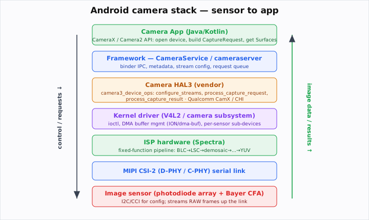
App (Camera2/CameraX)          ← builds CaptureRequests, owns output Surfaces
  ↓ ↑
Framework (cameraserver)       ← CameraService, binder IPC, request/result queue, metadata
  ↓ ↑
Camera HAL3 (vendor)           ← camera3_device_ops: configure_streams, process_capture_request,
  ↓ ↑                             process_capture_result   (Qualcomm: CamX / CHI)
Kernel driver (V4L2 subsystem) ← ioctl, DMA buffers (dma-buf/ION), per-sensor sub-devices
  ↓ ↑
ISP hardware (Spectra)         ← fixed-function pipeline (B1)
  ↓ ↑
MIPI CSI-2 receiver            ← deserializes the sensor stream
  ↓ ↑
Image sensor                   ← photodiodes + Bayer CFA; configured over I2C/CCI
Why it exists. Layering separates concerns and lets one Android framework run on any vendor's hardware via the HAL contract: apps and the framework are vendor-agnostic; the HAL + driver are vendor-specific (Qualcomm's CamX/CHI). The kernel driver owns the hardware (ISP, CSI, DMA); the HAL implements the pipeline policy; the framework manages requests/results and security.
Where you see it (Qualcomm). This is the literal architecture you'd work in. The cross-functional round probes how a setting (exposure) flows from app → framework metadata → HAL → driver → sensor register, and how a frame flows back up with result metadata. "How does the kernel communicate with user space / HAL?" (Reports 15, 35) is exactly this boundary.
Answer. "A camera app uses the Camera2 or CameraX API to open the device, configure output Surfaces, and submit CaptureRequests. Those go through the framework's cameraserver over binder to the vendor Camera HAL3, which implements camera3 ops — configure_streams, process_capture_request, process_capture_result. The HAL programs the kernel driver via ioctl; the driver owns the V4L2 sub-devices, the MIPI CSI-2 receiver, the ISP hardware, and DMA buffers, and configures the sensor over I2C. Control flows down — a request with settings becomes sensor exposure/gain and ISP config — and data flows up — RAW through the ISP into YUV frames plus result metadata returned in request order. On Qualcomm, the HAL is CamX/CHI driving the Spectra ISP."
Follow-ups / gotchas. HAL3 is request-driven and pipelined (multiple requests in flight; results returned in submit order). Binder is the IPC. DMA buffers (dma-buf/ION) are shared zero-copy across layers. Cross-link: kernel/V4L2/ioctl/DMA → 07_embedded_linux_kernel.md; binder IPC → 04_os.md.
Seen in: CleverPrep ("camera system architecture sensor→ISP→driver→HAL→framework"); Reports 15, 35, 46 (kernel↔user-space↔HAL); standard expectation.
G2 · Q: Explain the Android Camera2 API, HAL3, and the camera3 capture operations.¶
Frequency: 🔥🔥 Common (CleverPrep tip: "Understand Android camera architecture (Camera2 API, HAL3)").
Concept — the basis. Camera2 is Android's low-level camera API; HAL3 (the camera3 model) is the vendor interface beneath it. The model is request → result:
- The app builds a CaptureRequest describing one frame: target output Surfaces and a bag of settings (exposure, focus, AWB mode, etc. as camera metadata).
- It submits requests to a capture session; the framework forwards them to the HAL.
- The HAL's camera3_device_ops implements: configure_streams (set up the output buffer streams), process_capture_request (accept a request + its output buffers), and it returns frames asynchronously via process_capture_result (filled buffers + result metadata), plus a notify SHUTTER callback with the timestamp.
- The HAL is pipelined: several requests can be in flight (pipeline depth), and results are returned in the same order requests were submitted.
Example — request/result flow:
app: CaptureRequest{ surfaces=[preview,jpeg], AE=on, AF=auto, exp=..., ... }
  → session.capture(request)
  → HAL.process_capture_request(req, output_buffers)
  → (pipeline delay) HAL.notify(SHUTTER, frame#, timestamp)
  → HAL.process_capture_result(frame#, filled buffers, result metadata)   // in submit order
Why it exists. The old Camera1 API was a fixed black box; Camera2/HAL3 exposes per-frame control (manual exposure/focus/RAW, multiple simultaneous streams, burst) and a clean, pipelined, request-based contract so the framework and apps stay vendor-neutral while vendors implement the pipeline. This per-frame control is what makes computational photography (HDR/night burst control) possible.
Where you see it (Qualcomm). Qualcomm's HAL3 implementation is CamX with the CHI (Camera Hardware Interface) override layer for customization. Camera apps (incl. GCam ports) rely on Camera2 manual controls + RAW. The result-in-order, pipelined contract shapes the whole driver/HAL design.
Answer. "Camera2 is Android's low-level, per-frame camera API; HAL3 is the vendor interface under it, using a request-result model. The app builds a CaptureRequest — output Surfaces plus settings as camera metadata — and submits it to a capture session. The framework hands it to the HAL, whose camera3 ops are configure_streams, process_capture_request, and process_capture_result, with a notify SHUTTER callback. The HAL is pipelined: multiple requests in flight, results returned in submission order with result metadata. This per-frame control enables manual exposure, RAW, multiple streams, and bursts — the basis of computational photography. On Qualcomm it's implemented as CamX with the CHI override layer."
Follow-ups / gotchas. Pipeline depth / in-flight requests; results in order. Repeating request drives preview; capture() for stills/burst. Metadata is a tag/value bag (camera_metadata). Buffer management API (Android 10+) lets the HAL request buffers late. Cross-link: function-pointer ops table (camera3_device_ops) → 01_c_programming.md; binder/IPC → 04_os.md.
Seen in: CleverPrep ("Camera2 API, HAL3"); standard Android camera expectation.
G3 · Q: Design a camera driver architecture supporting multiple sensors.¶
Frequency: 🔥🔥 Common (CleverPrep: "Design a camera driver architecture supporting multiple sensors").
Concept — the basis. A phone has several sensors (wide, ultrawide, tele, front, depth), each with its own registers, Bayer order, calibration, and CSI-2 lane/data-type config — but they share the ISP and a common control flow. The design goal is a common core + per-sensor plug-ins: abstract everything sensor-specific behind a uniform interface (an "ops" table = function pointers / a driver model), so the framework drives any sensor through the same calls.
Example — the layered design:
        ┌─────────────── Camera HAL / framework (sensor-agnostic) ───────────────┐
        ▼
  ┌──────────────────────── Common camera/ISP core driver ──────────────────────┐
  │  request handling · ISP config · CSI-2 RX mgmt · DMA buffers · 3A plumbing   │
  └───────┬───────────────┬────────────────┬───────────────┬────────────────────┘
          ▼               ▼                ▼               ▼
   ┌────────────┐  ┌────────────┐   ┌────────────┐  ┌────────────┐
   │ sensor drv │  │ sensor drv │   │ sensor drv │  │ sensor drv │   ← per-sensor module
   │  WIDE      │  │ ULTRAWIDE  │   │  TELE      │  │  FRONT     │     implements ops:
   └────────────┘  └────────────┘   └────────────┘  └────────────┘     probe/init/
   (registers, Bayer order, gains, CSI lanes, calib tables differ per sensor)     start/stop/
                                                                                  set_exposure...
sensor_ops struct (function pointers) with the core; the core calls them uniformly. This is exactly the Linux V4L2 sub-device model (each sensor is a sub-device).
Why it exists. Without abstraction you'd duplicate the whole pipeline per sensor (unmaintainable). The ops-table pattern (polymorphism in C) lets you add a new sensor by writing one module implementing the interface — no changes to the core. It also cleanly handles per-sensor differences (Bayer order, calibration) that cause bugs (C5) if mishandled.
Where you see it (Qualcomm). Qualcomm's camera driver (CamX sensor modules / kernel sub-devices) is exactly this: a common core + per-sensor drivers. Routing N sensors over CSI-2 (virtual channels, muxing), sharing one or multiple ISP contexts, and concurrent multi-camera (e.g. wide+tele for zoom fusion) are the real design problems.
Answer. "I'd use a common core plus per-sensor plug-in modules. The core — sensor-agnostic — handles request processing, ISP configuration, the CSI-2 receiver, DMA buffer management, and 3A plumbing. Each physical sensor is a module that registers an ops table — probe, init, start/stop streaming, set_exposure, set_gain, set_focus — encapsulating its register map, Bayer order, CSI lane/data-type, and calibration tables. The core invokes any sensor through the same function-pointer interface, so adding a sensor is writing one module, not touching the core. This is the V4L2 sub-device model. The hard parts are routing multiple sensors over CSI-2 with virtual channels, sharing ISP contexts, and supporting concurrent multi-camera for zoom fusion — plus getting each sensor's Bayer order and calibration right to avoid color casts."
Solution / good example — the C ops-table abstraction:
#include <stdint.h>
struct sensor_ops {                                  // per-sensor function-pointer table
    int  (*probe)(void *ctx);                         // detect & identify (read chip ID)
    int  (*init)(void *ctx);                          // load register init sequence
    int  (*start_stream)(void *ctx);
    int  (*stop_stream)(void *ctx);
    int  (*set_exposure)(void *ctx, uint32_t exp_us, uint32_t gain);
    int  (*set_focus)(void *ctx, int lens_pos);
    void (*get_caps)(void *ctx, struct sensor_caps *out); // res, Bayer order, CSI lanes, calib
};
struct sensor_dev { const struct sensor_ops *ops; void *ctx; struct sensor_caps caps; };

// Core drives ANY sensor uniformly — no per-sensor branches:
int core_start(struct sensor_dev *s){
    if (s->ops->init(s->ctx)) return -1;
    return s->ops->start_stream(s->ctx);
}
// Registration: each sensor module fills a sensor_ops and registers with the core.
int register_sensor(struct sensor_dev *s);
Follow-ups / gotchas. Concurrency (locking when sensors share the ISP/CSI), hot-plug/probe, power sequencing (regulators/clocks per sensor), per-sensor calibration loading. The function-pointer ops table is the crux (same pattern as file_operations/camera3_device_ops). Cross-link: function pointers / ops tables → 01_c_programming.md; V4L2 sub-devices/kernel → 07_embedded_linux_kernel.md; this is also an LLD question → 10_lld_system_design.md.
Seen in: CleverPrep camera guide ("Design a camera driver architecture supporting multiple sensors"); Report 15 (multi-sensor/driver context); standard expectation.
G4 · Q: Design a low-latency camera preview pipeline for real-time display.¶
Frequency: 🔥🔥 Common (CleverPrep: "Design a low-latency camera preview pipeline for real-time display").
Concept — the basis. Preview must show the live scene with minimal latency (sensor photon → pixel on screen) and no stutter at 30/60 fps. The pipeline: sensor → CSI-2 → ISP → YUV frame → buffer → composite/display, all streaming and double/triple-buffered so producer (camera) and consumer (display) never block each other. Latency is minimized by: a lighter ISP path than capture (lower res, fewer/cheaper stages), zero-copy buffer sharing (dma-buf, no memcpy between stages), a shallow pipeline depth, VSync-aligned presentation to avoid tearing, and keeping the heavy work on fixed-function hardware (not the CPU).

Example — the preview dataflow:
Sensor → CSI-2 → ISP(light) → [buffer pool, N=2–3] → SurfaceFlinger/display, swap on VSync
         (no copies — dma-buf passed by handle; producer/consumer via a fence/queue)
Why it exists. High preview latency feels laggy ("the image trails my hand"); dropped frames stutter. Users judge a camera partly by preview smoothness. So preview trades some IQ for latency and steady frame rate, and uses buffer queues + VSync to keep producer and consumer decoupled and tear-free.
Where you see it (Qualcomm). The preview stream is one of several HAL3 output streams (preview + still + video), configured for low latency; it uses dma-buf and a buffer queue (BufferQueue/SurfaceFlinger) with fences. Power matters too — preview runs continuously, so it must be efficient.
Answer. "Preview is a streaming, multi-buffered pipeline tuned for latency and steady frame rate, not maximum IQ. Sensor data comes over CSI-2 into a lighter ISP path — lower resolution, fewer/cheaper stages than capture — producing YUV frames into a small pool of buffers, double or triple buffered so the camera producer and display consumer never block. I'd minimize latency with zero-copy buffer sharing via dma-buf (no memcpy between stages), a shallow pipeline depth, fixed-function hardware for the heavy work, and VSync-aligned presentation to avoid tearing. It's a producer-consumer pipeline with a buffer queue and fences; the still-capture path can be heavier because it's not in the live loop."
Solution / good example — buffer-pool / producer-consumer skeleton:
// Triple-buffered preview ring: camera fills, display drains; never blocks, no tearing.
#define NBUF 3
typedef struct { void *dmabuf[NBUF]; int fill; int show; } PreviewRing;

void on_isp_frame_done(PreviewRing *r){          // producer (camera/ISP completion)
    int next = (r->fill + 1) % NBUF;
    if (next != r->show) r->fill = next;          // advance if a free buffer exists
    // submit r->dmabuf[r->fill] to the display queue (by handle — zero copy)
}
void on_vsync(PreviewRing *r){                    // consumer (display, VSync-aligned)
    int next = (r->show + 1) % NBUF;
    if (next != r->fill) r->show = next;          // present newest ready buffer at VBlank
}
Follow-ups / gotchas. Double vs triple buffering (triple avoids producer stalls at cost of +1 frame latency). VSync prevents tearing (H1). Zero-copy (dma-buf) is the latency win. Don't run heavy NR/HDR in preview. Cross-link: screen tearing/buffers H1; producer-consumer/reader-writer sync → 04_os.md; dma-buf → 07_embedded_linux_kernel.md; LLD → 10_lld_system_design.md.
Seen in: CleverPrep camera guide ("Design a low-latency camera preview pipeline for real-time display"); standard expectation.
H. Display & video¶
H1 · Q: What is screen tearing, and how do you fix it with frame buffers?¶
Frequency: 🔥🔥 Common (Display-team Reports 2 & 6: the signature "design an algorithm to address screen tearing" LLD; producer/consumer + reader-writer sync).
Concept — the basis. Screen tearing happens when the display reads a frame buffer while it's still being written, so the top of the screen shows the old frame and the bottom shows the new one, split by a visible horizontal "tear" line. It's a producer-consumer / reader-writer race: the SoC (producer) writes the buffer; the panel (consumer) scans it out line-by-line at the refresh rate; if a write lands mid-scanout, you see two frames at once.
The fix — double buffering + VSync: keep two buffers. The producer renders into the back buffer while the display scans out the front buffer. Only swap them (flip pointers) during the VBlank interval (VSync — the gap between frames when nothing is being scanned out). The consumer therefore always reads a complete, consistent frame. Triple buffering adds a third buffer so the GPU/producer never stalls waiting for the swap (at the cost of one extra frame of latency).
Example — the Qualcomm display-team setup (from the reports):
CRT panel + SoC share ONE frame buffer; SoC=producer, panel=consumer; 120 FPS, 1 ms TAT.
Line-by-line scanout + mid-frame writes → tearing.
Fix: double-buffer; producer writes BACK; swap to FRONT only at VSync (reader-writer sync).
Why it exists. A single shared buffer can't be safely read and written at once — classic concurrency hazard. Double buffering + VSync serializes the hand-off so the reader never sees a partially-written frame. It's a direct application of producer-consumer and reader-writer synchronization (the OS topic the interviewer is really probing).
Where you see it (Qualcomm). The display/multimedia loop loves this question as an LLD: design the buffering + synchronization to eliminate tearing under a real-time deadline (120 fps, 1 ms turnaround). It connects display, camera preview (G4), and OS sync.
Answer. "Screen tearing is when the display scans out a frame buffer while it's still being written, so the screen shows part of the old frame and part of the new one split by a tear line — a producer-consumer race between the SoC writing and the panel reading. The fix is double buffering with VSync: the producer renders into a back buffer while the display reads the front buffer, and you swap them only during VBlank, so the display always sees a complete frame. Triple buffering adds a third buffer so the producer never stalls on the swap, trading one frame of latency. It's reader-writer / producer-consumer synchronization applied to frame buffers."
Solution / good example — the design (and where the full sync code lives):
Buffers: FRONT (being scanned out), BACK (being rendered).  [+ optional 3rd for triple buffering]
Producer (SoC):   render → mark BACK ready.
Sync point:       at VSync/VBlank, atomically swap FRONT↔BACK (page flip).
Consumer (panel):  always scan out FRONT (never mid-write).
Synchronization:   producer & consumer coordinate via the VSync signal + a fence/lock
                   (reader-writer / producer-consumer). Newest-ready wins to minimize latency.
04_os.md and 10_lld_system_design.md.)
Follow-ups / gotchas. VSync adds up to one frame of latency (the gaming "VSync on/off" trade-off); adaptive sync (VRR) is the modern fix. Double (min) vs triple (no producer stall, +latency). Tearing is fundamentally a sync problem. Cross-link: reader-writer/producer-consumer, mutex/semaphore → 04_os.md; full LLD → 10_lld_system_design.md.
Seen in: Display-team Reports 2 & 6 ("Design an algorithm to address screen tearing", "CRT panel + SoC share one frame buffer", "reader-writer synchronization"); standard display expectation.
H2 · Q: How can you control the bit-rate of video?¶
Frequency: 🔥 Occasional (JoinTaro Video Codec Report 8: "How can you control the bit-rate of video?").
Concept — the basis. Bit-rate is the data per second of encoded video (bits/s). Rate control is the encoder logic that hits a target bit-rate by adjusting how aggressively it compresses each frame — primarily the quantization parameter (QP) (coarser quantization → fewer bits, lower quality), plus frame-type/GOP choices. Modes: - CBR (constant bit-rate): hold a steady rate (for fixed-bandwidth channels like streaming/calls). Quality varies with scene complexity. - VBR (variable bit-rate): let the rate rise on complex scenes and fall on simple ones for more even quality at a target average. - CQP / constant-quality (CRF): fix quality (QP), let the rate float. - Capped VBR / ABR: VBR with a ceiling.
A rate-control loop tracks a bit budget (often modeled as a buffer — the HRD/VBV) and raises QP when ahead of budget / lowers QP when under, allocating bits across the GOP, frame, and macroblock levels.
Example — the control idea:
target_bits_per_frame = bitrate / fps
if (bits_used_so_far > budget)  QP++   // compress harder → fewer bits, lower quality
else                            QP--   // spend bits → higher quality
(allocate more bits to I-frames and complex frames; obey the VBV buffer to avoid under/overflow)
Why it exists. Networks and storage have limits; rate control fits the video into the available pipe/space while maximizing quality. The fundamental knob is QP (the quality↔size lever); the modes trade rate stability against quality stability.
Where you see it (Qualcomm). The hardware video encoder (Venus/codec block) implements rate control for camcorder, streaming, and video calls; choosing CBR vs VBR, target/peak bit-rate, and GOP/I-frame interval is exactly the multimedia tuning a codec engineer does within latency/quality budgets.
Answer. "Bit-rate is encoded bits per second, and you control it with rate control in the encoder, mainly by adjusting the quantization parameter — coarser quantization spends fewer bits at lower quality, finer spends more. The modes are CBR for a steady rate on fixed-bandwidth channels, VBR to let the rate float with scene complexity for more even quality at a target average, and constant-QP/CRF to fix quality and let the rate float. The rate controller tracks a bit budget, usually modeled as a buffer (VBV/HRD), and raises QP when it's over budget and lowers it when under, allocating bits across the GOP, frame, and macroblock levels — and giving more bits to I-frames and complex frames. You also tune GOP length and I-frame interval."
Follow-ups / gotchas. QP is the lever. CBR vs VBR trade-off (rate stability vs quality stability). VBV/HRD buffer prevents under/overflow (decoder buffer model). Two-pass VBR for offline. Resolution/frame-rate/GOP also affect size. Cross-link: codecs/GOP/I-P-B → H3; quantization → 09_computer_arch_digital_design.md.
Seen in: JoinTaro Video Codec Engineer (Report 8, "How can you control the bit-rate of video?"); standard codec expectation.
H3 · Q: How do video codecs work — H.264/HEVC, I/P/B frames, and motion estimation?¶
Frequency: 🔥 Occasional (Video Codec role, Report 8; "Video — codecs" in the patterns summary; cross-refs HDR/interpolation motion).
Concept — the basis. A codec (coder-decoder) compresses video by removing redundancy. Two kinds: - Spatial (intra) redundancy — within one frame (neighboring pixels are similar): handled by intra prediction + transform (DCT-like) + quantization + entropy coding, like JPEG. - Temporal (inter) redundancy — between frames (consecutive frames are similar): handled by motion estimation/compensation — find where each block moved from in a reference frame (a motion vector) and code only the small residual (difference), not the whole block.
Frame types in a GOP (Group of Pictures): - I-frame (intra): coded alone, no references — a full image, the random-access point. Largest. - P-frame (predicted): references previous frame(s); codes motion vectors + residual. Smaller. - B-frame (bi-predictive): references both past and future frames → best compression, but adds latency/reorder (decode order ≠ display order).
Example — a GOP:
display:  I  B  B  P  B  B  P ...
          └ I = full image; P = forward-predicted; B = predicted from both sides ┘
sizes:    I  >  P  >  B    (more references = smaller)
Motion estimation: for each block, search a reference frame for the best match → motion vector + residual.
Why it exists. Raw video is enormous (1080p30 YUV 4:2:0 ≈ 93 MB/s: 1920×1080×1.5 B/px × 30). Codecs cut this ~50–200× by exploiting that frames repeat in space and time. HEVC (H.265) roughly doubles H.264's compression at the same quality (bigger/flexible block sizes — CTUs up to 64×64, more prediction modes) at higher compute cost.
Where you see it (Qualcomm). The hardware codec block encodes camera video and decodes playback in real time within a power budget; the camera/codec interface is YUV 4:2:0. Motion estimation is the same primitive used in HDR/night alignment (D1/D3) and frame interpolation (D4). Rate control (H2) sits on top.
Answer. "Codecs compress video by removing spatial redundancy within a frame and temporal redundancy between frames. Within a frame it's intra prediction plus transform, quantization, and entropy coding, like JPEG. Between frames it's motion estimation: for each block, search a reference frame for the best matching block, store a motion vector and only the residual difference. Frames in a GOP are I-frames — self-contained, the random-access points and largest; P-frames — predicted from previous frames; and B-frames — predicted from both past and future, smallest but adding latency since decode order differs from display order. HEVC roughly doubles H.264's efficiency at the same quality using larger flexible coding units and more prediction modes, at more compute. Codecs operate on YUV 4:2:0, and motion estimation is the same idea as HDR alignment and frame interpolation."
Follow-ups / gotchas. Decode order ≠ display order with B-frames (reordering buffer). Motion search cost vs quality (block sizes 16×16 down to 4×4 in H.264; CTUs to 64×64 in HEVC). I-frame interval = seek granularity + error resilience. AV1/VP9 are royalty-free alternatives. Cross-link: rate control H2; motion estimation also in D1/D4; DCT/quantization → 09_computer_arch_digital_design.md.
Seen in: JoinTaro Video Codec Engineer (Report 8); "Video — codecs" pattern summary; standard codec expectation.
I. Qualcomm Spectra context¶
I1 · Q: What is the Qualcomm Spectra ISP, and why does it matter?¶
Frequency: 🔥 Occasional but expected — CleverPrep explicitly says "Research Spectra ISP."
Concept — the basis. Spectra is Qualcomm's Image Signal Processor integrated into the Snapdragon SoC — the dedicated hardware that runs the camera pipeline (B1) at phone power. Key facts (Snapdragon 8 Gen 1 generation): a triple 18-bit ISP (three parallel ISPs, one per concurrent camera), processing up to 3.2 gigapixels/second — enough for, e.g., 108 MP at 30 fps on one camera, or burst 240×12 MP/s. The 18-bit pipeline gives far more dynamic-range headroom than the previous 14-bit generation. It works with the camera DSP and the AI engine (the "Snapdragon Sight" / CV-ISP branding) for computational features: multi-frame HDR/night, semantic segmentation-based tuning, and ML denoise. The HAL/driver layer that programs it is CamX/CHI (G2).
Why it matters (for the interview). Knowing Spectra shows you understand where all the pipeline theory runs in Qualcomm's product, and why fixed-function hardware is necessary (a CPU can't do 3.2 Gpix/s at mobile power). It frames the IQ-vs-speed trade-offs (D5) in concrete terms — the throughput, bit depth, and concurrency are the budget you design within.
Where you see it (Qualcomm). Literally the silicon you'd be working on. Triple-ISP enables concurrent multi-camera (the multi-sensor driver of G3); 18-bit enables better HDR; the CV-ISP path enables real-time segmentation/ML in the camera.
Answer. "Spectra is Qualcomm's Image Signal Processor inside Snapdragon — the dedicated hardware running the camera pipeline at phone power. The Snapdragon 8 Gen 1 generation has a triple 18-bit Spectra ISP processing up to 3.2 gigapixels per second, so it can handle, say, 108 MP at 30 fps or three concurrent cameras, with 18-bit giving more dynamic-range headroom than the prior 14-bit design. It works with the camera DSP and AI engine — Snapdragon Sight / CV-ISP — for computational photography like multi-frame HDR, night mode, semantic segmentation tuning, and ML denoise, and it's programmed through the CamX/CHI HAL. It matters because that throughput and concurrency are exactly the budget the pipeline and multi-sensor driver must fit within, and it's why this work is fixed-function hardware rather than CPU."
Follow-ups / gotchas. Specs are generation-specific (the "triple 18-bit, up to 3.2 gigapixels/second" figure is the Snapdragon 8 Gen 1 (2021); the prior Snapdragon 888 was a 14-bit ISP at ~2.7 Gpix/s, and newer generations differ — state the generation when quoting). Triple-ISP = concurrency (multi-camera). 18-bit = dynamic range. Cross-link: multi-sensor driver G3; IQ-vs-speed D5; fixed-function HW → 09_computer_arch_digital_design.md.
Seen in: CleverPrep camera guide (tip: "Research Spectra ISP"); standard Qualcomm-context expectation.
§ Encyclopedia — searchable glossary¶
Every bold-italic term used above is defined here, alphabetically, with why it exists / where you see it and a micro-example. Use your editor's find (⌘F / Ctrl-F) to jump to a term.
3A — the three camera control loops: auto-exposure, auto-focus, auto-white-balance. Why/where: make the camera adapt to any scene automatically; driven by ISP statistics, feeding back to sensor/lens/ISP. Example: point at a sunset → AE darkens, AWB warms, AF locks.
ADC (analog-to-digital converter) — converts a photodiode's analog charge into a digital number, usually per sensor column. Why: the rest of the pipeline is digital. Where: sets RAW bit depth (10/12/14-bit).
Auto-exposure (AE) — feedback loop setting exposure time + gain (+aperture) to hit a target brightness from the histogram (C2). Gotcha: anti-flicker, damping to avoid oscillation.
Auto-focus (AF) — drives the lens to make the subject sharp via contrast (hill-climb) or PDAF (phase) (C3). Where: face-priority AF; hybrid AF.
Auto-white-balance (AWB) — neutralizes the illuminant's color cast by per-channel gains; classic gray-world assumes the scene averages to gray (C4). Gotcha: fails on single-color scenes.
Bayer CFA (color filter array) — the RGGB mosaic over sensor pixels (50% green, 25% R, 25% B) so each pixel measures one color (A1). Why: one sensor captures color cheaply; demosaic reconstructs the rest. Example: RAW = single-channel mosaic.
Bilinear interpolation — distance-weighted average of the 4 surrounding pixels for sub-pixel sampling/resize (E1); also the simplest demosaic. Why: smooth, cheap, separable. Contrast: bicubic uses 16 pixels (sharper, costlier).
Bicubic interpolation — fits a cubic over the 4×4 neighborhood; sharper than bilinear, ~4× cost, can ring/overshoot (E1).
Bit depth — bits per channel/sample (8-bit display, 10–14-bit RAW, Spectra 18-bit internal). Why: more bits = more dynamic range / less banding.
Black-level correction (BLC) — subtracts the sensor's dark pedestal so true black = 0 (B2). Where: early RAW stage; per Bayer channel. Gotcha: skip it → milky blacks, biased color.
B-frame (bi-predictive) — a video frame predicted from both past and future references → smallest, best compression, but adds latency (decode≠display order) (H3).
CBR / VBR — constant vs variable bit-rate rate-control modes (H2). Why: CBR for fixed channels (steady rate), VBR for even quality at a target average.
CCM (color-correction matrix) — 3×3 matrix mapping sensor RGB → sRGB, fixing cross-channel leakage (B4). Where: after WB/demosaic, before gamma. Gotcha: wrong CCM → color cast.
Chroma subsampling — storing color (chroma) at lower resolution than luma; 4:2:0 = chroma halved both ways, 1.5 B/px (F1). Why: eye resolves brightness > color → ~50% bandwidth saved.
CMOS / CCD — image-sensor technologies; CMOS (per-pixel/column readout, cheap, rolling shutter) dominates phones; CCD (charge shifted out) is legacy/scientific.
Codec — coder-decoder; compresses video by removing spatial (intra) + temporal (inter/motion) redundancy (H3). Examples: H.264/AVC, HEVC/H.265, AV1.
Computational photography — using multiple frames + computation to beat single-shot optics: HDR, night mode, super-resolution (D1/D3). Where: Snapdragon Sight.
Contrast-detection AF (CDAF) — focus by hill-climbing image contrast; accurate but slow and direction-blind (C3).
Convolution — sliding a kernel/mask over an image, weighted-summing neighbors; the engine of blur/sharpen/edge/CNN (E3). Note: convolution flips the kernel; correlation doesn't (same for symmetric kernels).
CSI-2 (MIPI Camera Serial Interface 2) — standard high-speed serial link sensor→ISP over D-PHY/C-PHY, multi-lane, with virtual channels (A3). Companion: slow I2C/CCI control bus.
Demosaic (debayer) — reconstruct full RGB from the Bayer mosaic by interpolating missing colors (B3). Gotcha: naive bilinear → zippering/false color → use edge-aware methods. The RAW→RGB boundary.
D-PHY / C-PHY — MIPI physical layers under CSI-2; D-PHY = clock+data lanes; C-PHY = 3-phase encoding (more bits/symbol) (A3).
Dynamic range — ratio of brightest to darkest a sensor/scene spans; limited by full-well (saturation) and read noise. Why HDR exists: one exposure can't span a high-DR scene.
Edge detection — finding large-gradient locations; Sobel (gradient kernels) or Canny (blur→Sobel→non-max-suppress→hysteresis) (E2). Where: sharpening, contrast AF, CV.
Face detection — locating faces; classic Viola–Jones (Haar + integral image + cascade) or CNN detectors (E4). Where: face-priority 3A, portrait.
Gamma correction — non-linear curve (in^(1/2.2)) converting linear light → perceptual/display encoding; saves bits, matches vision (B5). Late stage. Distinct from tone mapping.
Global shutter — all pixels expose simultaneously → no motion skew, but costly (A2). Contrast: rolling shutter.
GOP (Group of Pictures) — a codec frame group starting with an I-frame, then P/B frames (H3). Why: random access + compression; interval = seek granularity.
Gray-world — AWB assumption that the scene averages to gray → scale channels to equalize averages (C4). Gotcha: fails on dominant-color scenes.
HDR (high dynamic range) — capture/merge multiple exposures to exceed single-shot dynamic range (D1). Challenge: motion → ghosting → align + de-ghost.
HEVC (H.265) — codec ~2× more efficient than H.264 at equal quality via larger flexible CTUs + more modes, at higher compute (H3).
I-frame (intra) — self-contained video frame, no references; random-access point; largest (H3).
Integral image — precomputed prefix-sum image so any rectangle sum is O(1); enables real-time Viola–Jones face detection (E4). Tie-in: 2-D prefix sums.
Intra / inter prediction — codec prediction within a frame (spatial) vs from other frames (temporal/motion) (H3).
ISP (Image Signal Processor) — fixed-function hardware turning RAW Bayer into a clean RGB/YUV image via the pipeline (B1). Qualcomm: Spectra.
Lens-shading correction (LSC) — per-pixel gain map undoing lens vignetting + color shading (corners darker/tinted) (B2). Where: early RAW stage; radial or mesh.
Local tone mapping (LTM) — region-varying tone mapping that preserves local contrast (B5); brightens a dark face without blowing the sky.
Luma / chroma — brightness (Y) vs color (Cb/Cr) components of YUV (F1). Why split: subsample chroma, keep luma full-res.
Masking — either a convolution kernel (filter) or a binary/region map selecting pixels to process (E3). Where: portrait/ROI effects.
MIPI — the standards body; here CSI-2 (camera) over D-/C-PHY (A3).
Motion estimation — finding where a block moved (a motion vector) between frames to code only the residual (H3); also used in HDR/night alignment and frame interpolation (D1/D4).
Multidimensional image — image data beyond 2-D: color (channel axis), video (time), volume (depth), hyperspectral (bands), ML tensor (N×C×H×W) (E6). Gotcha: stride/pitch and HWC vs CHW layout.
Night mode — many-frame low-light fusion: align + average (SNR↑√N) + HDR/denoise/tone-map (D3). Why: accumulate light over time without long-exposure blur.
NV12 / NV21 / I420 — YUV 4:2:0 memory layouts; I420 planar (Y,U,V), NV12 semi-planar (Y + interleaved UV), NV21 = NV12 with U/V swapped (F1). Gotcha: NV12↔NV21 swap → green/purple cast.
Otsu's method — automatic threshold that maximizes between-class variance for segmentation (E5).
PDAF (phase-detection AF) — paired/dual-pixel sensors measure phase disparity → direction + distance to focus in one fast step (C3). Gotcha: weak in low light/low texture.
P-frame (predicted) — video frame predicted from previous frame(s); motion vectors + residual; smaller than I (H3).
Photodiode — the sensor's light-to-charge element (a "photon bucket"); colorblind, hence the Bayer CFA (A1).
Quad Bayer — sensor CFA with 2×2 same-color groups; bins in low light (sensitivity) or re-mosaics for full res in good light (A1).
Quantization parameter (QP) — the codec's main quality↔size lever; higher QP = coarser, fewer bits (H2).
Rate control — encoder logic hitting a target bit-rate by adjusting QP and bit allocation, modeled with a VBV/HRD buffer (H2). Modes: CBR/VBR/CQP.
RAW — the sensor's unprocessed, single-color-per-pixel, linear-light Bayer data before the ISP (A1, B1). Why process in RAW: BLC/LSC/WB need linear, per-channel data.
Rolling shutter — row-by-row exposure/readout; cheap CMOS default but causes motion skew/jello and flicker banding (A2). Impact: complicates HDR alignment.
Segmentation — partitioning an image into regions/classes; classic (threshold/watershed/k-means) or deep (semantic/instance/panoptic) (E5). Where: portrait, region tuning.
Sharpening — edge-based local-contrast boost (often unsharp masking) late in the pipeline (B1, E3).
Sobel — 3×3 gradient kernels (Gx, Gy) for edge detection; |G|=√(Gx²+Gy²) (E2). Step 2 of Canny.
Spectra — Qualcomm's Snapdragon ISP (triple 18-bit, up to 3.2 Gpix/s on 8 Gen 1) running the camera pipeline; "Snapdragon Sight" computational features (I1).
Stride / pitch — bytes per image row, possibly > width×bytes-per-pixel due to alignment padding (E6). Gotcha: a top source of garbled images/casts.
Temporal NR — denoise by averaging a pixel across frames; great on static scenes, needs motion gating to avoid ghosting (D2).
Tone mapping — compress high-dynamic-range data into the display range; global (one curve) or local (per-region) (B5). Distinct from gamma.
VBV / HRD — the decoder buffer model the rate control must respect to avoid under/overflow (H2).
Vignetting — lens-caused corner darkening, fixed by LSC (B2).
Virtual channel — CSI-2 mechanism to multiplex multiple logical streams (image + metadata + PDAF) on one link (A3).
Viola–Jones — classic real-time face detection: Haar features via integral image + AdaBoost cascade (E4).
VSync / VBlank — the display's vertical-blanking interval where buffer swaps happen to avoid screen tearing (H1, G4). Trade-off: up to one frame of latency.
White balance — see auto-white-balance; per-channel gains (diagonal), vs CCM which is cross-channel (3×3).
YUV / YCbCr — color space separating luma (Y) from chroma (Cb/Cr), enabling chroma subsampling (F1). Where: ISP output, preview, all video codecs.
Zippering — demosaic artifact (alternating light/dark along edges) from interpolating across edges; fixed by edge-aware demosaic (B3). Sibling artifact: false color.
§ Last-5-minutes cheat sheet¶
- Sensor: photodiodes (colorblind) + Bayer CFA RGGB (50% green = luminance) → single-channel RAW. Rolling shutter (row-by-row, skew) vs global (all at once). Link = MIPI CSI-2 (data) + I2C/CCI (control).
- ISP pipeline: RAW domain → black-level → lens-shading → defect/RAW-denoise → white balance → DEMOSAIC → RGB domain → noise reduction → CCM (3×3 → sRGB) → gamma/tone-map → sharpen → RGB→YUV 4:2:0. Principle: linear/Bayer fixes before demosaic; color/perceptual after.
- 3A: AE (histogram → exposure time + gain; damp, anti-flicker), AF (contrast hill-climb vs PDAF phase = one fast jump), AWB (gray-world: scale R,B so avgR=avgG=avgB).
- Green tint debug: bisect the pipeline; suspects = Bayer order, AWB gains, black-level/LSC, CCM, NV12/NV21 U-V swap. RAW green → sensor side; only displayed green → downstream/format.
- HDR: bracket short/mid/long → align → per-pixel merge → tone-map. Challenge = ghosting (motion) → de-ghost. Night mode = many frames + align + average (SNR↑√N).
- Noise reduction: spatial = bilateral (edge-preserving, weight by intensity too); temporal = average over frames + motion gating. Over-denoise → plastic look. IQ vs speed/power/thermal.
- Interpolation: bilinear (4 px, cheap) vs bicubic (16 px, sharp). Frame interp needs motion/optical flow or it ghosts.
- Edges: Sobel Gx/Gy →
|G|=√(Gx²+Gy²); Canny = blur→Sobel→non-max-suppress→hysteresis. Convolution = slide kernel/mask. - Color: RGB (3 B/px) vs YUV 4:2:0 (1.5 B/px, one chroma per 2×2) — eye sees luma > chroma → ~50% saved. Codecs/preview use YUV.
- Stack: App (Camera2) → framework (cameraserver/binder) → HAL3 (camera3 ops: configure_streams / process_capture_request / process_capture_result; Qualcomm CamX/CHI) → kernel driver (V4L2, ioctl, dma-buf) → ISP → CSI-2 → sensor. Request→result, pipelined, results in order.
- Multi-sensor driver: common core + per-sensor ops table (function pointers) = V4L2 sub-device model. Low-latency preview: light ISP path, double/triple buffer, zero-copy dma-buf, VSync.
- Tearing: reader/writer race on a shared frame buffer → double-buffer + swap at VSync (front/back); triple = no producer stall.
- Video: bit-rate controlled via QP (CBR/VBR/CQP, VBV buffer). I (alone) / P (past) / B (both) frames in a GOP; motion estimation = vector + residual. HEVC ≈ 2× H.264.
- Spectra: Qualcomm Snapdragon ISP — triple 18-bit, up to 3.2 Gpix/s (8 Gen 1); fixed-function HW + DSP/AI for computational photography.
Evidence base: qualcomm_camera_interview_experiences.md. Frequencies are approximate (sample = 75 reports; the camera/ISP domain questions come largely from the CleverPrep aggregated guide + JoinTaro/GfG camera reports). Diagrams in assets/ (cam_*.svg). Cross-references: pure C/pointers/memory → 01_c_programming.md · C++/OOP/RAII → 02_cpp_oop.md · algorithm complexity (KMP/BFS/sort) → 03_dsa.md · OS sync (mutex/semaphore/reader-writer), scheduling, virtual memory, binder IPC → 04_os.md · CNN/ResNet/R-CNN/YOLO/optical-flow ML → 06_ml_deeplearning.md · kernel/V4L2/ioctl/DMA/dma-buf drivers → 07_embedded_linux_kernel.md · aptitude/puzzles → 08_logical_puzzles_aptitude.md · bit depth/DCT/quantization/fixed-function pipeline hardware → 09_computer_arch_digital_design.md · screen-tearing & buffer LLD, multi-sensor design → 10_lld_system_design.md · project/behavioral framing → 11_behavioral_hr_projects.md.